
Image deblurring reconstructs a sharper image from observations described by a blur model. In the linear model, a matrix or linear operator mixes values of the unknown image; measurement noise perturbs the observed result. The inverse problem must therefore recover attenuated distinctions while controlling amplification of measurement noise, as the two-pixel example illustrates.
For and , a differentiable graph is invariant precisely when . This is the chain rule along a trajectory on the graph. The equation determines coefficients in a local power-series approximation of a stable manifold or unstable manifold; checking tangent directions alone does not ensure invariance.
G2 phase follows completed nuclear DNA replication and precedes mitosis. The ordinary diploid state is . [ref]
During S phase, nuclear DNA replication produces paired sister chromatids. DNA content rises from to , while the chromosome count remains .
During G1 phase, growth and preparation precede DNA replication. The ordinary diploid nuclear state is .
The Lyman-alpha forest is the multitude of foreground Lyman-alpha absorption features in a distant quasar's spectrum, at wavelengths shorter than its own redshifted Lyman-alpha emission. The quasar supplies a bright background; intervening neutral hydrogen atoms remove photons near their local Lyman-alpha line resonance. Many dips can therefore come from one atomic transition encountered at different redshifts, rather than from many different chemical elements. Some features are instead transitions of other ions, so a dip alone does not identify Lyman-alpha absorption. This makes faint foreground gas detectable through the light it removes, even when its own emission would be difficult to see. [ref]
https://ned.ipac.caltech.edu/level5/Sept01/Rauch/Rauch1.html. Rauch (1998), The Lyman Alpha Forest in the Spectra of QSOs, section 1
.Ignoring peculiar velocity for the moment, an absorber at cosmological redshift puts its Lyman-alpha line atThe rest wavelength is in the ultraviolet; at it appears at in the optical spectrum. In a toy sightline to a quasar at , absorbers at appear at , all shortward of the quasar's Lyman-alpha emission position . The absorbing atoms see the selected photons at their own resonance; the observed dip's redshift belongs to the foreground gas. Peculiar velocity adds a Doppler shift, so the inferred is not a pure distance coordinate. The rest wavelength and resonance interpretation are given in Rauch (1998), section 1.
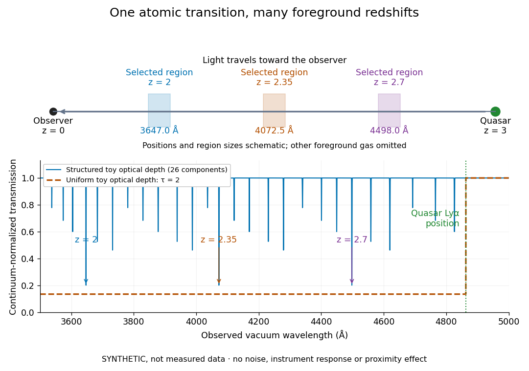

The diagram uses invented optical depths and 26 Doppler cores; three selected foreground regions are marked. Their drawn positions and sizes are schematic. The dashed comparison imposes a uniform optical depth , giving transmission throughout the chosen foreground band. It is an idealized smooth-absorption model, not a measured spectrum or a prediction of the actual intergalactic medium.
The smooth comparison explains the Gunn-Peterson effect: neutral hydrogen distributed throughout an expanding intergalactic medium can absorb continuously over a wavelength interval, because different parts of the path resonate with different observed wavelengths. The resolved Lyman-alpha forest instead has strong transmission fluctuations and distinguishable absorption lines. These need not represent isolated compact clouds: diffuse sheets and filaments in the cosmic web can generate peaks in optical depth along one line of sight. A continuously varying gas distribution can look like a collection of lines. [ref]
https://ned.ipac.caltech.edu/level5/Sept01/Rauch/Rauch1.html. Rauch (1998), section 1: smooth absorption
. [ref]https://ned.ipac.caltech.edu/level5/Sept01/Rauch/Rauch5_1.html. Rauch (1998), section 5.1: synthetic sightlines and extended structures
.An early observation makes the identification concrete. Lynds's 1971 paper analyzed six spectrograms of the quasar 4C 05.34, with emission redshift , taken in spring 1970 using an image-tube spectrograph on Kitt Peak's 84-inch telescope. Five covered – with approximately resolution; the most informative covered about – at resolution. Its reproduced spectrogram shows the strong Lyman-alpha emission flanked mostly on the short-wavelength side by numerous absorption lines. Lynds tabulated their wavelengths and estimated strengths, identified five absorption redshift systems, and proposed that many remaining unidentified lines were the same Lyman-alpha line at additional redshifts. He explicitly warned about blending, an incomplete census of weak lines, and wavelength errors around –. The result established a striking spectral pattern; the paper's proposed interpretation did not measure a separate physical cloud for every dip. [ref]
https://adsabs.harvard.edu/pdf/1971ApJ...164L..73L. Lynds (1971), The Absorption-Line Spectrum of 4C 05.34, Figure 1, Table 1 and discussion
.A contrasting observation demonstrates smooth, very strong absorption. Becker and collaborators (2001) used the Echelle Spectrograph and Imager on Keck II to observe the quasar SDSSp J103027.10+052455.0 at . Sky lines gave an instrumental full width at half maximum of about near , or spectral resolving power . After sky subtraction and flux calibration, the mean continuum-normalized transmission over – was , consistent with zero; this corresponds to absorption redshifts approximately –. They identified a Gunn-Peterson trough. Crucially, resonant Lyman-alpha absorption is so sensitive that even a small neutral fraction can make transmission undetectable: the trough alone does not establish a mostly neutral intergalactic medium or uniquely date reionization. [ref]
https://arxiv.org/pdf/astro-ph/0108097. Becker et al. (2001), sections 2–4: instrument response, transmitted flux and interpretation
.What a spectrum constrains is a radiative transfer problem. For an ideal foreground screen with negligible emission into the observed beam, the intrinsic continuum-normalized transmission isHere is spectral radiative flux, is its unabsorbed continuum, is optical depth, is neutral hydrogen number density, and is neutral hydrogen column density along proper path length . A Voigt profile model constrains redshift, column density and a velocity width together. A nearly black line has lost much of its sensitivity to further increases in optical depth; blending and an uncertain continuum can also admit different fitted components. Finite spectral resolving power and noise limit which widths and weak features can be measured. [ref]
https://ned.ipac.caltech.edu/level5/Sept01/Rauch/Rauch2.html. Rauch (1998), section 2: resolution, noise and profile analysis
. [ref]https://arxiv.org/pdf/astro-ph/0101005. Kim, Cristiani and D'Odorico (2001), section 3: fitted parameters and nonunique profile fits
.For a purely thermal Doppler core, use the velocity convention . The Maxwell-Boltzmann velocity distribution then giveswhere is the Boltzmann constant, is temperature and is a hydrogen atom's mass. This is times the Gaussian distribution's standard deviation. Higher temperature spreads the same column density over more velocities. An instrument also broadens a line: locally, for a nearly flat continuum, the recorded transmission is approximately the convolution of with the normalized instrumental response, not the exponential of a convolved optical depth. A Gaussian response with full width at half maximum has standard deviation , where is the speed of light and the spectral resolving power.
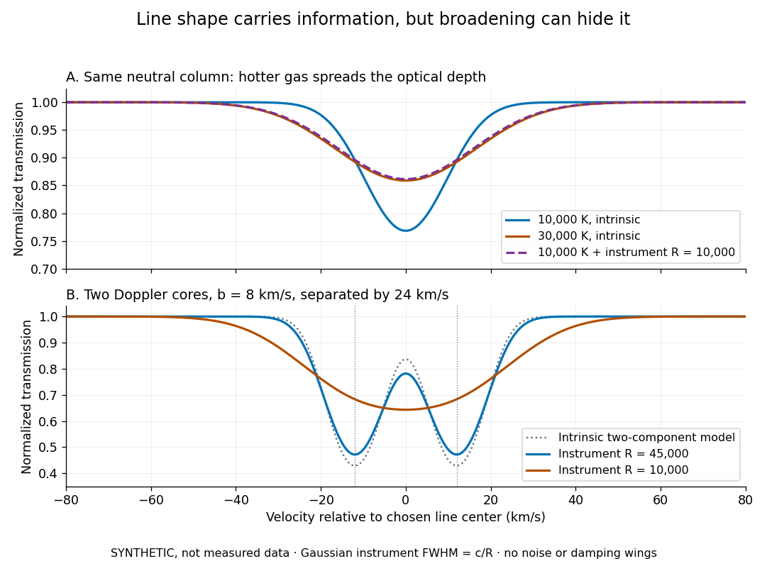
Synthetic absorption profiles: thermal broadening, instrumental smoothing and unresolved blends
. Details. 
The upper model fixes the integral , hence the neutral hydrogen column density for this transition, while changing temperature. A cooler line blurred by an instrument resembles a warmer intrinsic line. The lower model has two equal Doppler cores separated by : reducing spectral resolving power merges them into one apparent feature. Both panels use invented profiles, Gaussian instrumental responses, and no noise or damping wings. They illustrate an inverse problem, rather than measurements of temperature or a universal relation between a dip and a cloud.
Better observations provide the inputs to that inverse problem. Kim, Cristiani and D'Odorico (2001) analyzed three quasars with the VLT's UVES spectrograph. For HE2217–2818, Table 1 records and of exposure in the – setup in October 1999. Isolated thorium-argon lamp lines measured ; the data were resampled into bins, with signal-to-noise ratios about – per pixel over –. They fitted a local polynomial continuum, fitted Voigt profiles, and compared statistics of the transmitted flux. Their analysis excluded the region near the quasar to avoid the quasar proximity effect and used the interval between its Lyman-beta and Lyman-alpha emission to reduce confusion with other Lyman-series absorption. Features below became confused with noise, setting their adopted lower column density limit. Figure 1 shows the measured spectrum, fitted profiles and residuals. This was a calibrated absorption measurement, with explicit selection limits. [ref]
https://arxiv.org/pdf/astro-ph/0101005. Kim, Cristiani and D'Odorico (2001), UVES observations, sections 2–3, Table 1 and Figure 1
.Even after instrumental correction, a width need not be purely thermal Doppler broadening. Hubble flow across extended gas, peculiar velocity structure and unresolved blends can contribute. If an isolated line's intrinsic width obeys with an independent Gaussian nonthermal contribution , then ; gives a computed upper bound about . A complex blend need not satisfy this single-component model. Noise can also bias the fitted widths of weak lines. This is why the thermal cutoff of Lyman-alpha line widths, calibrated against gas models, is more informative than assigning a temperature to every dip. [ref]
https://ned.ipac.caltech.edu/level5/Sept01/Rauch/Rauch3_3.html. Rauch (1998), section 3.3: width measurements, noise bias and bulk motions
.Finally, neutral hydrogen column density is not total gas mass density. In a pure hydrogen approximation, with gas optically thin to ionizing radiation and nearly fully ionized in photoionization equilibrium, the Lyman-alpha forest photoionization scaling giveswhere counts all hydrogen nuclei, is the photoionization rate, is the radiative recombination coefficient and is the neutral fraction. At fixed temperature and , doubling quadruples ; doubling halves it. These computed examples explain both the sensitivity to density contrast and the ambiguity: stronger absorption can mean denser gas, weaker ionizing radiation, a different temperature, or more path length. The Jeans-length ionization correction for the Lyman-alpha forest adds a size model rather than an independently measured depth. Optically thick Lyman limit systems and damped Lyman-alpha systems require different treatment. [ref]
https://ned.ipac.caltech.edu/level5/Sept01/Rauch/Rauch5.html. Rauch (1998), section 5: neutral fraction and ionization correction
. [ref]https://arxiv.org/pdf/astro-ph/0104272. Schaye (2001), section 2 and Appendix equations A6–A7: ionization balance and the Jeans-length model
.The beauty of the Lyman-alpha forest is that a spectrum converts otherwise faint foreground gas into a sequence of markers through cosmic time. With a model of radiative transfer, velocities, ionizing radiation and the temperature-density relation of photoionized intergalactic gas, its transmission statistics probe the cosmic web and gas thermal history. A single line of sight remains one narrow sample, not a unique three-dimensional density map. [ref].
The cosmic ionizing background is the diffuse radiation field capable of photoionization of intergalactic gas. Its specific intensity depends on source luminosity functions, ionizing photon escape fractions, cosmological redshifting, and radiative transfer through absorbers. Quasars and star formation supply major contributions with different spectral shapes and evolution.
Diffuse gas in photoionization equilibrium is often approximately described by the displayed temperature-density contrast relation. Photoheating and expansion cooling produce its thermal history. It is an empirical model for low-density gas, not the adiabatic equation of state of every intergalactic phase. Lyman-alpha forest line widths constrain both the temperature at a reference density and the slope through their lower envelope.
The Weierstrass transform is Gaussian convolution, . It smooths appropriate functions and is the heat semigroup at unit time. The Brownian transition semigroup uses variance- Gaussian kernels and therefore supplies the scaled time family.
A linear integral equation depends linearly on its unknown function. For example, with has a trivial homogeneous null space whenever its inhomogeneous problem has a unique solution: otherwise a nonzero homogeneous solution could be added to that solution. This is the uniqueness step used in dressing constructions of a Lax pair.
This square-root-kernel integral equation is inverted by integrating over and interchanging integrations. The inner integral over equals , so . Differentiating recovers . The changes of variables , put the angular-ray equation into this form.
A permutation assigns facilities to locations, and the objective combines their pairwise interactions with pairwise location costs. Ordered-pair and unordered-pair conventions differ by a factor of two for symmetric data. The decision version is NP-complete: letting record a directed cycle makes the objective exactly the length of a travelling salesman problem tour under the ordering given by the permutation. The optimization version is NP-hard.
Given bidders' values for item bundles, the winner determination problem maximizes over disjoint allocated bundles. When every item must be assigned, the bundles form a partition. General values permit complements and difficult combinatorial search; monotone submodular set functions permit a greedy half-approximation. Complexity claims must specify whether the values are supplied explicitly or by a value oracle.
If , has an integer solution, with variables and all data bounded by , it has one satisfying the displayed bound. Apply support-minimal rays of a nonnegative kernel to in the cone . Its integer generators have coordinates bounded by . Generators with positive last coordinate normalize to feasible points with coordinates at most ; their coefficients form a convex combination. The remaining generators are integer recession directions. Subtract the integer parts of their coefficients from the original integer solution. The result remains integral and feasible and has coordinates at most . Its binary length is polynomial in the input size. Splitting unrestricted integer variables and adding integer slacks reduces general integer linear feasibility to this form, proving its membership in NP.
A congruence of squares says that two integers have the same square modulo a positive integer . Factoring their difference of squares givesA useful integer factorization results when or is a proper divisor of . Divisibility of a product does not generally force divisibility of either factor by all of : different prime factors of can divide different parts of that product.
For , . ThereforeThus . The prime seven divides the difference, while eleven divides the sum. These computations already give a complete prime factorization because seven and eleven are prime numbers.
The Chinese remainder theorem explains the hidden sign choices. The four congruence classes solving have representatives . Modulo seven each is or ; modulo eleven each is or . Two independent sign choices produce four roots. The inputs thirteen and twenty agree modulo seven and disagree by sign modulo eleven, allowing their sum and difference to separate the two prime factors.
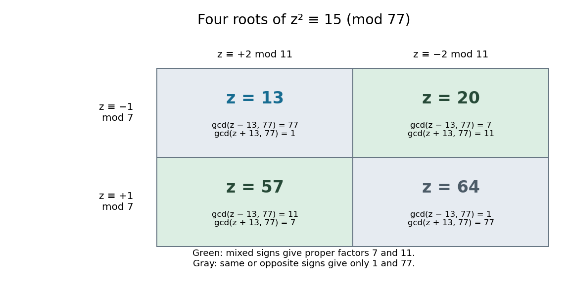

For distinct odd prime numbers , and , a solution with and modulo yields both proper factors by the two greatest common divisors. For a general composite integer, a proper divisor need not itself be prime; further factoring can remain. If or in the coprime case, the two calculations return and one instead. A factor base helps generate relations, but does not ensure every resulting relation is useful.
For historical context, Pomerance describes Kraitchik's 1920s enhancement of the difference-of-squares approach associated with Fermat: seek a difference that is a multiple of , rather than exactly . His account also notes antecedents in Gauss and Seelhoff, so this is not an attribution of the whole idea to a single inventor. [ref]
https://math.dartmouth.edu/~carlp/PDF/paper109.pdf. Carl Pomerance, A Tale of Two Sieves (1996), pp. 1474–1475: difference-of-squares and congruent squares
.The odd part of a positive integer is the unique odd positive integer obtained by repeatedly dividing by two. The process terminates because the positive integers decrease. If with odd, then would make even and would make even; hence and . Two positive integers have the same odd part exactly when their ratio is an integral power of two. The odd positive integers therefore give representatives for the resulting equivalence classes.
A factor base is a finite set of small prime numbers over which selected auxiliary integers are completely factored. Some methods also record a sign coordinate for , which is not a prime number. A positive integer supported entirely on the chosen factor base gives an exponent vector; reducing that vector modulo two records which prime exponents are odd integers. The product is a square of a number precisely when every prime exponent is an even integer.
For the original toy , use factor base and the two relationsThe residues have exponent vectors and in the order . Adding the two vectors modulo two gives , so multiplying the residues gives . Consequentlyand and . Neither individual residue was a square; combining the relations made all exponents even.
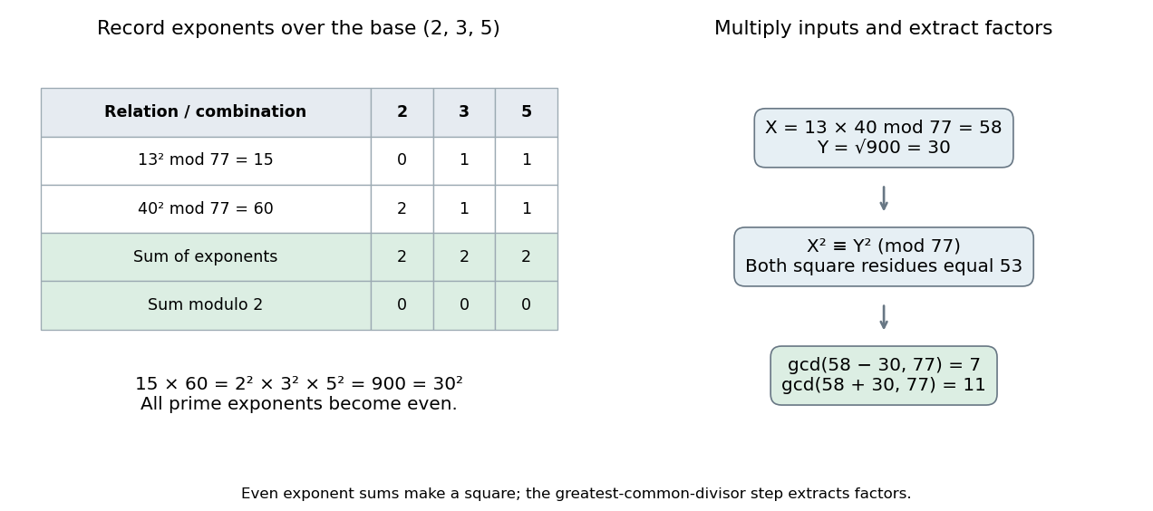

In a larger collection, choose relations with positive residues . If a nonempty selection has an even sum in every exponent coordinate, setThen . Finding such a selection is a linear dependence problem over the finite field : the indicator vector of the chosen relations belongs to the kernel of a linear map given by the parity matrix. This is why a problem about prime factors recruits linear algebra. The final congruence of squares may still be trivial, so another selection can be needed. [ref]
https://crypto.stanford.edu/pbc/notes/crypto/factoring.html. Ben Lynn, Factoring and Discrete Logarithms, Dixon's Algorithm: exponent matrix and kernel
.There is a tradeoff: a small factor base gives a smaller parity matrix, but fewer auxiliary integers factor completely over it. A larger factor base accepts more relations but makes the linear algebra larger. Negative auxiliary values need an additional sign coordinate, and a selected product needs even sign parity as well as even prime exponents. Pomerance's account explains this balance and the historical development of combining smooth relations; the toy example omits algorithm-specific sieving and running-time claims. [ref]
https://math.dartmouth.edu/~carlp/PDF/paper109.pdf. Carl Pomerance, A Tale of Two Sieves (1996), pp. 1475–1476: exponent parity, factor bases and signs
.A repdigit is a positive integer whose base- expansion repeats one nonzero digit . For , and , the finite geometric series gives . For example, has decimal digits, all equal to five.
Every prime number not dividing divides infinitely many such repdigits. If it divides , every length works. Otherwise, if it does not divide , the Fermat little theorem gives divisibility for lengths that are multiples of , and division by is justified by its modular inverse. If , the sum is congruent to modulo , so lengths divisible by work instead. A prime dividing but not divides none, since . This distinction prevents invalid cancellation of the geometric-sum denominator.
Lossless source coding encodes source messages so they can be recovered exactly. Shannon's source coding theorem relates its achievable average code length to information entropy.
There are unlisted articles, also show them or only show them.