Chlorophyll is a family of molecules that absorb light for photosynthesis. In chloroplasts, chlorophyll works with proteins in thylakoid membranes; absorbing light initiates energy capture rather than directly constructing a sugar. See OpenStax Biology 2e, 8.2: photosynthetic pigments.
Phase folding of a light curve maps timestamps onto a trial cycle of duration . Given a reference time , define the phase in cycles bywhere is the fractional part, using the floor function also for negative . Plot brightness against rather than ; measurements separated by an integer multiple of occupy the same phase. For a periodic function , this reveals the shared shape of many cycles. Folding changes coordinates; it neither averages samples nor chooses the correct by itself. Welsh et al.'s folded Kepler plot separates the exoplanet transit and orbital brightness modulation. [ref]
https://www.ucolick.org/~jfortney/papers/Welsh10.pdf. Welsh et al. (2010), figure 1
.The second figure uses a completely synthetic trapezoidal dip: days, day, and the same depth and four-hour duration as the first figure. Different colours identify four successive cycles. Correct folding superimposes the dips; a wrong trial orbital period spreads them out. If , the centre of the th repeated event shifts by approximately cycles when folded on , for . With days, the fourth plotted event is displaced by cycles. Transit-timing variations can also smear a constant-period fold, so retain the original timestamps and inspect individual events.
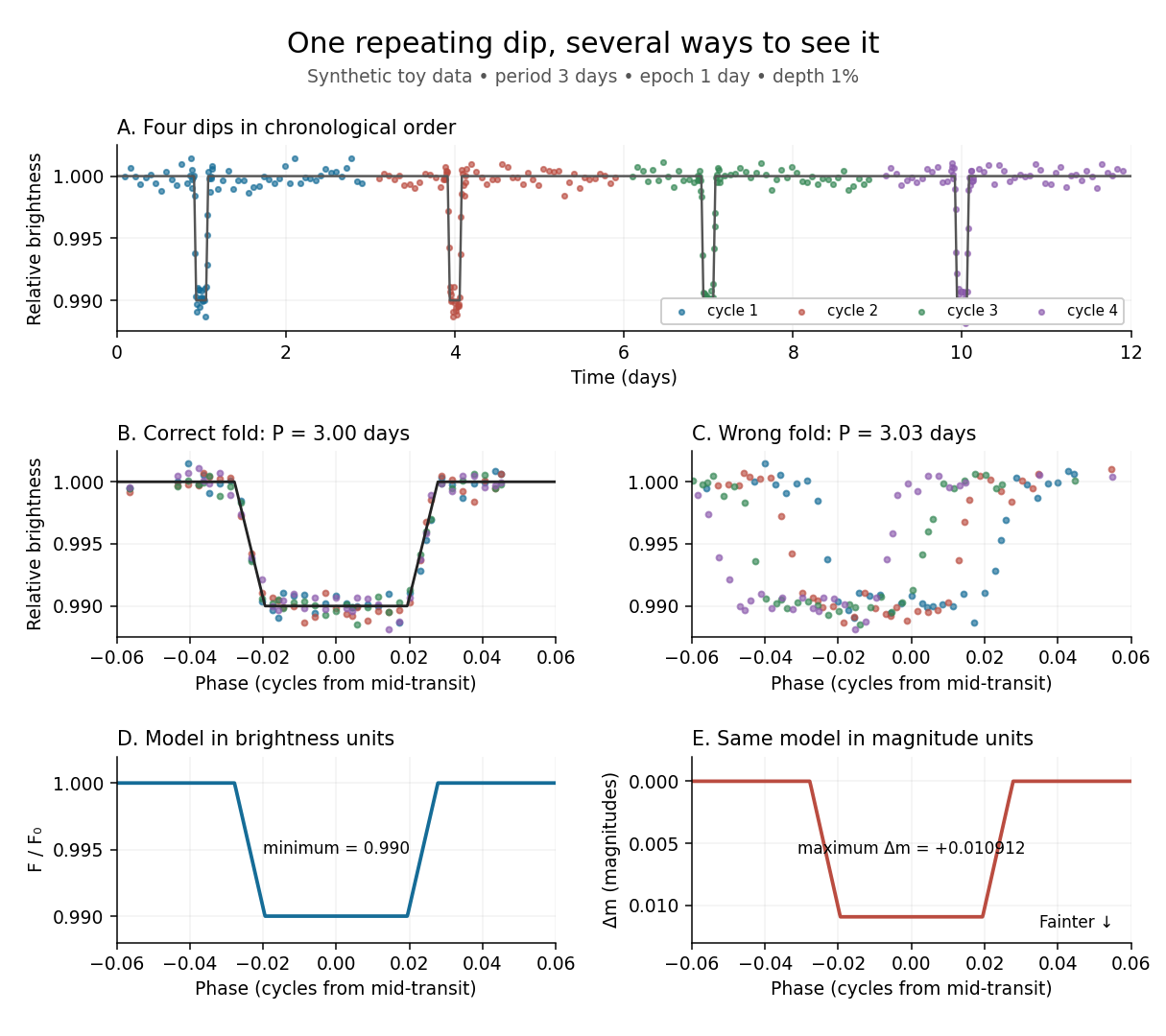
Toy phase folding: repeated synthetic dips align at the correct period; a flux dip becomes a positive magnitude change
. Details. One may combine nearby phases with a weighted mean, but the uncertainty reduction requires assumptions. For independent measurements with common standard deviation and effectively the same expected brightness within the bin, their arithmetic mean has standard deviation . Thus sixteen independent -precision samples give precision on that phase-bin mean. Shared calibration errors, changing starspots, and bins wide enough to mix ingress with out-of-transit brightness violate these assumptions. A folded plot can conceal changes between cycles. Gaussian process models can represent correlated variability and interpolate irregular samples, but their predictions and uncertainties depend on their assumed covariance function.
The bottom panels show the same model as relative brightness and as magnitude difference in one fixed photometric passband with a fixed magnitude zero point:A dip to gives magnitudes: fainter means a larger apparent magnitude. The figure places larger magnitude differences lower on the page so the two dip shapes are easy to compare; reversing that plotting convention does not change the formula. For and small , expansion of the logarithm gives . The exact transform is nonlinear: transforming an exposure's mean brightness is generally different from averaging its instantaneous apparent magnitudes. The ordinary logarithm cannot be applied to a nonpositive background-subtracted measurement; keep such measurements and their uncertainties in brightness units for an appropriate statistical model.
An exposure-averaged light curve models what a finite exposure measures. For a constant response during an exposure of duration , centred at , the expected mean brightness isThe integral has units of brightness times time; division restores the units of . Observed points fluctuate around this mean. A response that changes during the exposure must instead be included inside the integral, as in the first figure's known drift. Exposure duration and the interval between samples are distinct: there may be dead time or missing exposures.
A short dip can be blurred even with perfectly noiseless measurements. For a toy rectangular dip of fractional depth and duration , an exposure containing the whole dip has fractional depth : averaging hides part of its depth. A dip lasting ten minutes therefore appears only deep in a thirty-minute exposure. No interpolation recovers its shape from that single number without additional assumptions. Forward modelling should average the predicted light curve over each exposure before comparing it with the measurements. Kipping's analysis of exoplanet transit photometry demonstrates how ignoring this averaging biases inferred system parameters. [ref]
https://arxiv.org/abs/1004.3741. Kipping (2010), Binning is sinning
.Aperture photometry estimates brightness by summing calibrated detector pixels in an extraction region and subtracting the estimated background in that region. For equally weighted pixels, let be their total accumulated signal in electrons, the estimated background electrons per pixel over the same exposure, and the exposure duration. Then is a background-subtracted electron rate. Kepler applied aperture photometry to calibrated pixels with a fitted sky background. [ref].
This measurement trades source collection against background: enlarging the extraction region can retain more starlight but includes more sky brightness and neighbouring sources. Photon shot noise, read noise, and uncertainty in background subtraction contribute to its uncertainty. Dividing by a consistently measured reference rate gives a dimensionless light curve; it does not supply an absolute observed radiative flux. If contaminating light remains, the reference includes it and the inferred exoplanet transit depth suffers transit dilution.
In the first toy figure, the source's reference rate is electrons per second, the summed sky contribution is electrons per second, and a known multiplicative response is with in hours from mid-transit. The artificial exoplanet transit depth is , its total duration four hours, and its flat-bottom duration hours; the straight ingress and egress are a toy approximation, not an exact exoplanet transit photometry model. Each synthetic sample averages a -hour exposure and adds seeded normal distribution noise with relative standard deviation . Subtracting the known sky rate and dividing by the known response and reference rate recovers the dip. Real observations require estimating those corrections and carrying their uncertainty.
An optical pulse is a finite-duration envelope of light. A nearly monochromatic pulse has many carrier oscillations within its duration : in units with light speed one, its wavelength obeys . A slowly varying propagation-time map stretches the pulse duration by its derivative and divides the observed frequency by the same factor.
// Target: general-relativity.bigb
The pressure coefficient compares a local static pressure with a specified reference static pressure, using a fixed reference dynamic pressure:The reference mass density, speed, pressure and location must accompany a reported pressure coefficient. Keep the same throughout a surface distribution; replacing it by local gives a different quantity and fails at a stagnation point. The definition itself requires neither Bernoulli's principle nor inviscid flow, so measured pressure coefficients remain useful when those idealizations fail.
Positive means ; zero means equality; negative means . This sign does not specify the sign of absolute pressure. For stipulated absolute and , gives absolute: a deficit, not a negative absolute pressure. If equals atmospheric pressure, the numerator is gauge pressure; a wind tunnel's reference static pressure need not equal room atmospheric pressure. These are reference choices, not different physical pressures.
Under the same-height, constant-mass density , steady flow and inviscid flow hypotheses of the Bernoulli equation, and with the same Bernoulli invariant as the reference flow,The first equation immediately gives the second after subtracting and dividing by . Hence a lossless stagnation point has , gives , and gives . For a real stationary wall satisfying the no-slip boundary condition, the velocity is zero right at the wall; inserting that wall velocity in an inviscid flow formula would wrongly predict everywhere. A thin boundary layer approximation instead relates the wall pressure to the outer-flow pressure and uses the outer velocity where the Bernoulli equation applies.
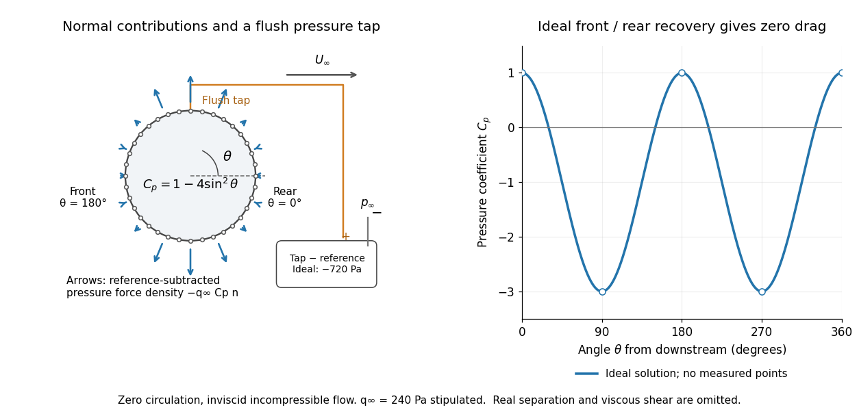
For potential flow around a circular cylinder of radius with zero circulation, the surface tangential velocity is . Thus the ideal pressure coefficient isWith measured from downstream, the front is at and the rear at zero. Both ideal stagnation points have , while the sides at and have . This exact model is a useful baseline for an experiment; its complete rearward pressure recovery is not a prediction for a separated real fluid wake.
To obtain a force, integrate the local normal contributions with their directions. Let be the unit normal vector from the body into the fluid and its closed wetted surface:The second equality removes a spatially constant reference pressure over the closed surface; it does not remove a nonuniform hydrostatic pressure or justify dropping the reference term on an isolated open patch. A negative contributes outwards in this reference-subtracted calculation, even though a positive absolute pressure still pushes inwards locally. Project onto the chosen lift and drag directions. The full fluid force also includes from the viscous stress tensor, including tangential shear stress; pressure tapping does not measure that contribution.
For the two-dimensional cylinder, force per unit span follows from per unit span and :Substituting gives : opposite points have identical pressure coefficients and opposite normal vectors. Zero drag despite a strongly nonuniform pressure is the instructive limitation associated with D'Alembert's paradox. Real viscosity, boundary layers and flow separation can prevent rearward pressure recovery and produce pressure drag. Thus the measured curve can test the model and estimate a pressure contribution without proving that total drag vanishes.
A motivating measurement is Virginia Tech's Experiment 3 - Flow Past a Circular Cylinder. Its open-jet wind tunnel holds a rotatable cylinder with end plates and 36 one-millimetre pressure tappings at ten-degree intervals. A reference Pitot-static tube supplies and to one digital manometer; a second connects a surface tap to its positive port and reference static pressure to its negative port. Record the simultaneous readings:The last equality uses the low-speed stopping relation, not an additional speed measurement. The manual requires sealed tubing and zero checks with the tunnel off. It also provides a water-column manometer: read each column's initial level, and subtract the independently measured reference-to-atmosphere pressure from the tap-to-atmosphere readings. Record tap positions after rotation. Compare the two instruments and check spanwise uniformity; end plates do not guarantee two-dimensional flow. [ref]
The inferential distinction matters: the manometers directly measure pressure differences, the ratio estimates pressure coefficients, and a surface integral estimates the pressure part of the force. Measure room absolute pressure and temperature if converting the reference difference to speed through the ideal gas law ; use thermodynamic temperature in that equation. For force reconstruction, cover the complete contour and use numerical integration with the tap geometry. Finite tap spacing, unknown end effects, probe disturbance and fluctuations limit that reconstruction; tubes and instruments also average or delay changing pressures. Retain the signed raw readings, repeated readings and reference readings so that these limits can be assessed. A small reference difference magnifies any zero error in the ratio, rather than producing a reliably large .
The signed lift divided by dynamic pressure times a stated reference area. For a two-dimensional airfoil, use instead. Reference area and experimental flow conditions are part of the definition of a reported coefficient; see lift for a worked scale and a pressure/balance experiment.
The octet rule is a useful empirical guide: many Lewis structures of chemical compounds containing carbon, nitrogen, and oxygen give each of those chemical atoms eight electrons when nonbonding electrons and all incident bonding electrons are counted. Hydrogen instead normally counts two electrons. These are local counts, not independent budgets: a shared bond pair counts at both endpoints but only once in the molecule's valence electron total.
In water, oxygen counts electrons; in Ammonia, nitrogen counts ; in , carbon counts and each oxygen counts . The charge-separated carbon dioxide drawing also satisfies the octet rule, so the octet rule alone cannot select the dominant contributor. Formal charge provides another check.
The octet rule is a heuristic rather than a theorem about every chemical bond. Odd valence electron totals cannot be partitioned entirely into electron pairs, and some valid Lewis structures have fewer or more than eight electrons around a chemical atom. See Chemistry 2e, 7.3: exceptions to the octet rule. The capacity of the and electron subshells, , helps motivate the guide for these chemical elements, but does not prove universal compliance. Lewis discussed a stable outer group of eight, together with a two-electron arrangement for hydrogen, in The Atom and the Molecule (1916), pp. 768 and 774.
A single nitrate Lewis structure singles out one N=O connection, yet the three N–O chemical bonds of the isolated symmetric ion are equivalent. Chemical resonance reconciles that symmetry with the integer electron pair allocations of a Lewis structure. The equal chemical bond lengths in nitrate are discussed in The Open University, Discovering chemistry: resonance structures.
Chemical resonance uses several Lewis structures with the same chemical atom connections and total electric charge to describe electronic structure that one allocation cannot fully express. The chemical atoms stay in place; the positions of bond pairs, lone pairs, and formal charges differ between drawings. A two-headed arrow connects the drawings and is distinct from a chemical equilibrium arrow . See the IUPAC Gold Book, resonance form.
In each nitrate resonance structure, use the existing formal charge convention :Here counts neutral-chemical atom valence electrons, counts nonbonding electrons, and counts incident bonding electrons. The sum is , agreeing with the nitrate ion's net electric charge. The formal charge rules and their distinction from actual atomic electric charge are given in Flowers et al., Chemistry 2e, 7.4: formal charges and resonance.
Keep one labelled oxygen fixed while reading the three nitrate resonance structures. Its connection is double in one drawing and single in two. Equal weighting within this three-contributor Lewis structure model gives the average bond orderThe same calculation applies to all three N–O connections. Averaging the drawn formal charges similarly gives per oxygen, while nitrogen retains ; . These fractions summarize the chosen contributors. They are not a measurement of partial atomic charge, a literal fraction of an electron sitting on an oxygen, or time spent in one drawing.
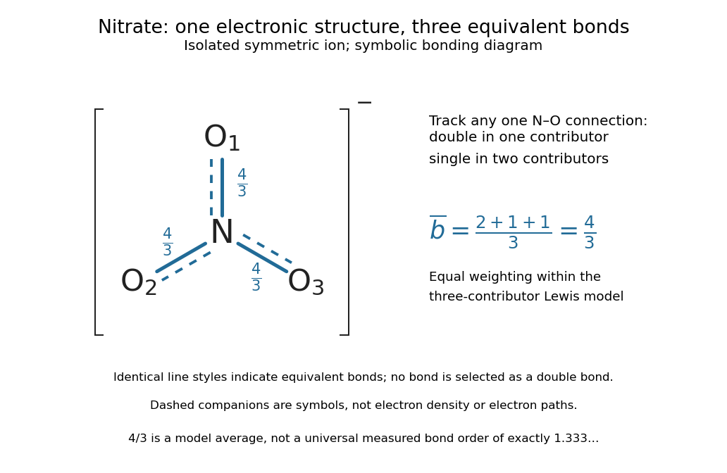
The resonance hybrid has one spatially continuous electron density extending over the ion. None of its N–O chemical bonds is permanently selected as the double connection of one contributor. The dashed marks above are symbols; electrons do not travel along them or make the marks float between chemical atoms. For isolated symmetric nitrate, symmetry makes the three N–O chemical bonds equivalent; an environment that distinguishes the oxygen sites can remove that equivalence. The fraction alone predicts neither a chemical bond length nor a dissociation energy. The general relation between multiple chemical bonds, lengths, and strengths is discussed in 7.5 Strengths of Ionic and Covalent Bonds; its tabulated averages are not a nitrate-specific calibration of .
Ozone provides a useful two-contributor comparison. Its valence electrons give three bond pairs and six lone pairs. One resonance structure has a double O–O connection on the left and a single one on the right; the other reverses these allocations while retaining the same chemical atom positions and connections. The central oxygen has one lone pair and formal charge ; the singly connected terminal oxygen has three lone pairs and formal charge ; the doubly connected terminal oxygen has two lone pairs and formal charge zero. Thus electrons and zero net electric charge are conserved. The equal-contributor bond order count is for either connection. See MIT 5.111, lecture 10, pp. 4–5: ozone resonance structures.
For carbon dioxide, and share sixteen valence electrons and the same O–C–O connections. The mirror drawing is also possible. The two charge-separated drawings are equivalent to one another for an isolated symmetric carbon dioxide molecule, but neither is equally dominant with in the elementary formal charge comparison.
Chemical resonance does not mean that a molecule rapidly flips between drawings, nor that separate molecules at chemical equilibrium carry the individual drawings. The actual electron density belongs to one combined electronic description. In a quantum mechanics treatment, contributors enter a linear combination of many-electron wavefunctions; a molecular orbital treatment can describe the extended electronic arrangement through molecular orbitals. The drawings alone provide neither a measured density nor numerical weights. Their usefulness is to expose the limitations of one localized allocation without pretending that every algebraically allowed Lewis structure contributes equally.
The formal charge of a chemical atom in a Lewis structure assigns it all of its nonbonding electrons and half of the electrons in its connections:Here is the neutral chemical atom's valence electron count, is the number of nonbonding electrons assigned to it, and is the number of bonding electrons incident on it. Count electrons, not electron pairs: two lone pairs mean , and two double connections mean . The number gives electric charge in units of the positive elementary charge. Equal splitting is a bookkeeping convention, regardless of the actual electron density. See the IUPAC Gold Book, formal charge.
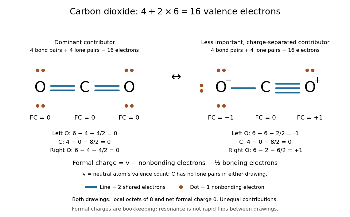
Sixteen valence electrons in two carbon dioxide Lewis structures: has zero formal charges, while has separated formal charges
. The first Lewis structure has two lone pairs on each oxygen. The second has three lone pairs on the singly connected oxygen, one on the triply connected oxygen, and none on carbon. Both use four bond pairs and four lone pairs; both satisfy the octet rule. Their contributions to chemical resonance are unequal, and the drawn formal charges are not partial atomic charges. Details.For , each oxygen has , , , giving formal charge . Carbon has , , , giving formal charge . For , the left oxygen has formal charge , carbon still has formal charge zero, and the right oxygen has formal charge . The net electric charge is zero in either drawing.
The Lewis structure with no separated formal charges is the dominant contributor in this elementary comparison; the charge-separated drawing is a less important contributor, rather than an equally dominant alternative. This is a qualitative selection rule, not a calculation of energy or numerical chemical resonance weights. See Flowers et al., Chemistry 2e, 7.4: comparing carbon dioxide structures. A zero formal charge does not imply zero partial atomic charge: the latter depends on partitioning the actual electron density, which a Lewis structure does not supply.
As a short consistency derivation, summing over all chemical atoms counts every drawn electron once: a nonbonding electron is assigned once, and a bonding electron contributes half at each of its two endpoints. Thuswhere is the total drawn valence electron count. The right side is the net electric charge in units of elementary charge. This catches a wrong budget even when individual octet rule checks look plausible.
A lone pair is an electron pair assigned to one chemical atom without a connecting line to another chemical atom in a Lewis structure. It is usually shown as two dots. Water has two lone pairs on oxygen, accounting for four valence electrons; Ammonia has one lone pair on nitrogen, accounting for two. In , each oxygen has two lone pairs, and carbon has none.
A lone pair can be reactive. In protonation of Ammonia, the nitrogen lone pair becomes a new bond pair to a proton:The proton supplies no electron, so the eight valence electrons are retained: three bond pairs plus one lone pair become four bond pairs. The resulting nitrogen has formal charge ; each hydrogen has formal charge zero. This is why identifying an available lone pair helps explain the chemical base behaviour of Ammonia, rather than merely decorating its formula.
Lewis already used the Ammonia to example in The Atom and the Molecule (1916), pp. 777–778. In modern terms the dots identify an allocation of electrons, not two stationary particles or an isolated patch unaffected by the rest of the molecule. A molecular orbital description can spread electronic amplitude over several chemical atoms while a localized Lewis structure remains useful for acid-base chemistry.
A bond pair is an electron pair allocated to a connection between two chemical atoms in a Lewis structure. A single line stands for one bond pair, or two electrons. A double connection contains two bond pairs, or four electrons; a triple connection contains three bond pairs, or six electrons. A bond pair is shared bookkeeping for the combined arrangement, rather than two distinguishable electrons each permanently owned by one endpoint.
In water, two bond pairs use of the eight valence electrons. In Ammonia, three bond pairs use of the eight valence electrons. In , each C=O connection contains two bond pairs, so there are four bond pairs in the entire carbon dioxide molecule. Counting connections and counting bond pairs therefore give different answers for multiple connections.
The same bond pair is treated differently for different questions: both endpoints count its two electrons for the octet rule, whereas each endpoint receives just one electron for formal charge. Neither convention asserts equal physical electron density at the endpoints. For electronic shapes, occupancy, and energy, see molecular orbital theory rather than treating a bond pair line as an entire wavefunction.
The VSEPR model predicts approximate molecular geometry by arranging the electron domains around a central chemical atom to reduce their mutual repulsion. Start with a Lewis structure, count the domains, and then distinguish the resulting electron pair geometry from the positions of the chemical atoms themselves. A lone pair counts as a domain even though it is not another chemical atom.[ref]
https://ocw.mit.edu/courses/3-091-introduction-to-solid-state-chemistry-fall-2018/g9v8zj6VObw_transcript.pdf. MIT 3.091, lecture 11: Lewis structures, domains and molecular shapes
Three worked counts have the same total of eight valence electrons. In methane, carbon's four plus the contributions of four hydrogen chemical atoms give : four bond pairs, no lone pairs, and tetrahedral molecular geometry. In Ammonia, nitrogen's five plus three from hydrogen give : three bond pairs and one lone pair, producing trigonal pyramidal molecular geometry. In water, oxygen's six plus two from hydrogen give : two bond pairs and two lone pairs, producing bent molecular geometry. All three have four electron domains; their molecular geometries differ.
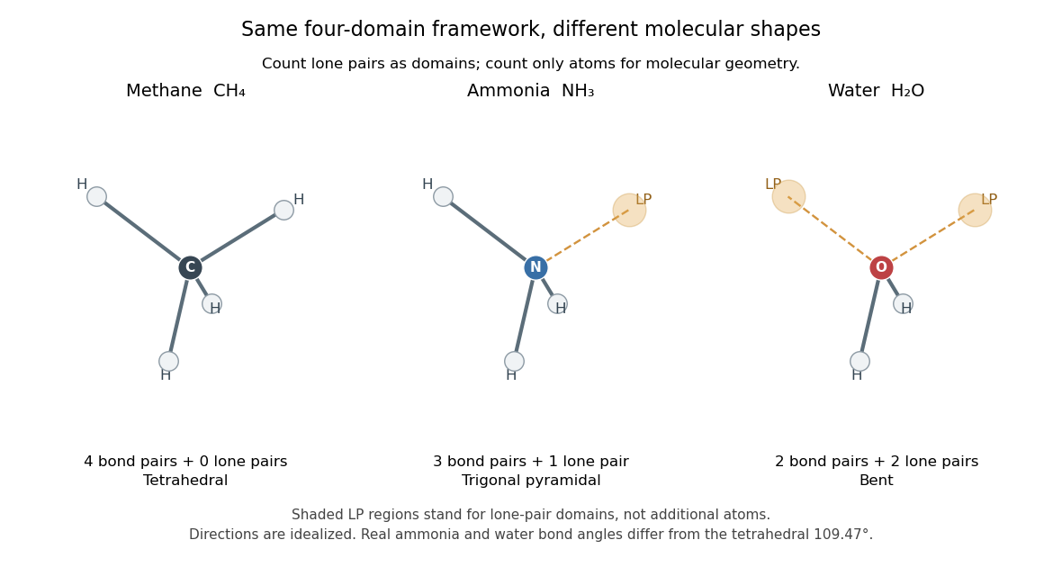


The regular tetrahedral directions can be represented by the unit vectorsEach pair has dot product , so the ideal bond angle is . This is a geometric calculation, rather than a prediction that every four-domain molecule has that exact bond angle. Lone pairs and different kinds of chemical bonds distort the ideal arrangement; water's H–O–H angle is about .[ref]
The model is attractive because small-number bookkeeping produces a spatial prediction without first solving for every molecular orbital. Shape then helps explain chemical polarity and which hydrogen bond donor or hydrogen bond acceptor sites are accessible. It is a qualitative model, not a full calculation of the electronic energy or a universal solution for every chemical compound. Gillespie and Nyholm's 1957 review [ref]
https://doi.org/10.1039/QR9571100339. Inorganic stereochemistry, Quarterly Reviews 11, 339–380
is a historical anchor for its development. Constant-input firing rate of a leaky integrate-and-fire neuron by  Codex 0 Created 2026-10-14 Updated 2026-11-05
For , reset and no explicit refractory interval, define and . Constant current givesThe threshold is approached only asymptotically at . At large current, . Adding an absolute neuronal refractory period changes the denominator to and makes the firing rate saturate rather than grow without bound.
For and Higgs multiplication , setWrite , , , where . Direct expansion gives . Its vanishing for every complex is therefore equivalent to , the Bogomolny equations. It is a parameter-dependent zero-curvature representation.
For the normalization points , and spatial infinity, the Volterra integral equation kernel is . Its lower entry in column one has factor ; column two has the opposite factor. With quadrants numbered counterclockwise, the column domains are , and , respectively.
Let have diagonal entries and off-diagonal entries and . Let have diagonal entries and off-diagonal entries . Substitution into the isomonodromic deformation compatibility identity gives the displayed equations on domains with . Thus , so and , a rescaled zero-parameter Painlevé II equation when . The leading coefficient is required by cancellation of the quadratic spectral terms.
For the modified Korteweg-De Vries equation with linear part , the Volterra integral equation kernel is . In column one its off-diagonal modulus is ; column two has the reciprocal modulus. Define by signs , by , by and by . The normalization points , and give column domains , and , respectively. Finite-path eigenfunctions can be entire at fixed coordinates while failing to be bounded outside these spectral sectors.
The meromorphic function has simple poles of residue one at . Subtracting removes all poles inside radius . Comparing its inner Taylor coefficients with the outer Laurent expansion gives annular coefficient . On circles of radius , the function is uniformly bounded: outside the strip use the exponential modulus, and inside it the imaginary part stays near an odd multiple of . The Laurent coefficient integral bounds , proving the sum.
There are unlisted articles, also show them or only show them.