Given finitely encoded linear inequalities, a maximum feasible subsystem is a largest collection that can be simultaneously satisfied. Its decision version asks whether some inequalities admit a common solution. This is NP-complete, despite polynomial time feasibility testing for each fixed collection. For a graph, use nonnegative variables , constraints for vertices, and copies of for each edge. A subsystem of size must retain a copy of every edge constraint and at least vertex constraints; those vertices form an independent set. Conversely an independent set of size supplies such a feasible subsystem by its indicator vector.
The ellipsoid method repeatedly asks a separation oracle about the center of a containing ellipsoid and replaces that ellipsoid by a smaller one containing its intersection with a separating half-space. The volume decreases by a dimension-dependent factor at each iteration. For rational polyhedra, the exact feasibility theorem has polynomial bit complexity in the dimension and coefficient encoding bounds when separation is polynomial time. It includes lower-dimensional feasible sets through rational precision bounds or suitable relaxations; one must not declare infeasibility just because the original feasible set has zero volume.
A nonempty linear polyhedron with integer inequality coefficients and right sides bounded by contains a point with the displayed bounds. Intersect with an orthant containing a feasible point. Moving along directions annihilating the active constraints, until another constraint becomes active, produces a vertex: the orthant prevents a whole nontrivial line from remaining feasible. At that vertex, choose independent active inequalities, including coordinate constraints as necessary. Cramer's rule and the Hadamard determinant inequality bound both determinants by . The resulting rational witness has polynomial binary length and is verifiable in polynomial time, proving that integer linear feasibility is in NP.
The set of minimizers of a linear objective on a linear polyhedron. It is a face: if a strict convex combination of two feasible points minimizes the objective, both points must also minimize it. Hence an extreme point of an optimal face is an extreme point of the original polyhedron. Successively minimizing further linear objectives restricts to nested faces, whose vertices remain original vertices. This preserves uniform rational denominator bounds in exact feasibility-oracle optimization.
A surplus variable converts a lower-bound inequality into , with . This is the lower-bound counterpart of a slack variable. When the original coefficients, right-hand side and decision variables are integer, the surplus variable is integer as well; that fact permits it to appear in an all-integer Gomory fractional cut row.
This form of linear programming additionally has the uniform vector as a strictly positive feasible point and known optimum zero. A homogeneous self-dual embedding of a linear program, followed by elimination of unrestricted Lagrange multipliers and normalization by the sum of nonnegative coordinates, yields this form without presupposing feasibility of the original program. The known start and optimum support projective interior-point methods. Polynomial bit-complexity statements additionally require finite rational input encoding; bounded arbitrary real coefficients alone do not provide it.
For a stimulus-conditioned Inhomogeneous Poisson process, the event log-likelihood is the displayed expression. A causal filter expansion can be fitted by maximum likelihood estimation, with a smoothness or size penalty and held-out validation. The integral term penalizes predicted spikes that did not occur; fitting only stimulus values at observed spikes omits this essential part.
For , the determinant is zero for every , even when one perturbation component is arbitrarily large. Linearized metric theory instead requires the eigenvalues of relative to the background spatial metric to be small, equivalently all its components in a background orthonormal frame to be small. The determinant of then expands as , and the volume element as .
Longitudinal displacement in linear dust perturbations by  Codex 0 Created 2026-10-14 Updated 2026-10-20
Mass conservation in a Lagrangian dust displacement gives , hence to first order. The perturbing gravitational potential determines the longitudinal part of the force, so the displayed equation holds for the curl-free displacement under the usual homogeneous boundary convention. A divergence-free transverse displacement instead satisfies . Taking the divergence gives without assuming the full displacement is longitudinal. The background Poisson equation with positive source requires .
The density power spectrum records the squared Fourier-mode amplitude, up to the chosen statistical normalization. Scale dependence acquired from primordial amplitudes and subsequent growth determines its spectral shape.
In a spatially flat universe containing separately conserved pressureless matter and a coasting fluid with , the ratio is proportional to the scale factor. If the coasting component is modeled by the barotropic fluid perturbation equations with no anisotropic stress, its contribution to the trace gravitational source vanishes because . The matter growing mode isA decaying solution is . The reduction of order formula with integrating factor produces the integral solution. It has during matter domination and tends to during coasting-fluid domination. Thus growth freezes rather than continuing in proportion to the scale factor. The background geometry is flat despite the same background expansion law as an open dust universe.
Expansion-weighted derivative of a passive density perturbation by Codex 0 Created 2026-10-14 Updated 2026-10-20
Codex 0 Created 2026-10-14 Updated 2026-10-20When the self-gravity source in the pressureless linear cosmological density perturbation equation is negligible, . Multiplication by makes it , so . This explains how Hubble friction changes growth for an arbitrary positive scale factor. For , the nonconstant mode is when and when .
The orbital overlap of normalized real atomic orbitals is their inner product . It is a dimensionless measure of their common amplitude, not an electron count. For the Gaussian function toy, increasing from to reduces from to . As tends to zero, both LCAO normalization denominators tend to .
An axis-angle representation specifies a rotation of three-dimensional Euclidean space by an oriented unit axis and an angle. The axis is fixed, and the perpendicular plane undergoes a pure rotation, with no dilation.
The permanent of a matrix adds the products obtained by choosing one entry in each row and one in each column. For an matrix with entries in the real numbers or complex numbers,Here each permutation chooses column in row , and the symmetric group lists every such bijection. The formula resembles the Leibniz formula for determinants, but omits the sign of a permutation. For a two-by-two matrix,The absence of alternating signs makes the permanent of a matrix particularly useful for counting allowed assignments.
For a zero-one matrix, let rows represent people, columns represent jobs, and mean that person can do job . This is the biadjacency matrix of a bipartite graph. A product in the permanent is one exactly when all the selected assignments are allowed; otherwise it is zero. Each surviving permutation assigns every person a different job, which is a perfect matching. Thus the permanent counts perfect matchings. This interpretation and the definition are given in Yufei Zhao, Probabilistic Methods in Combinatorics, §10.2, pp. 178–179.
For a fully enumerated example, takeAmong the six permutations of three columns, exactly three give nonzero products: , and . These tuples list the chosen column in each successive row. Each product is one, so . Their permutation signs are , giving . The diagram displays all three allowed assignments.
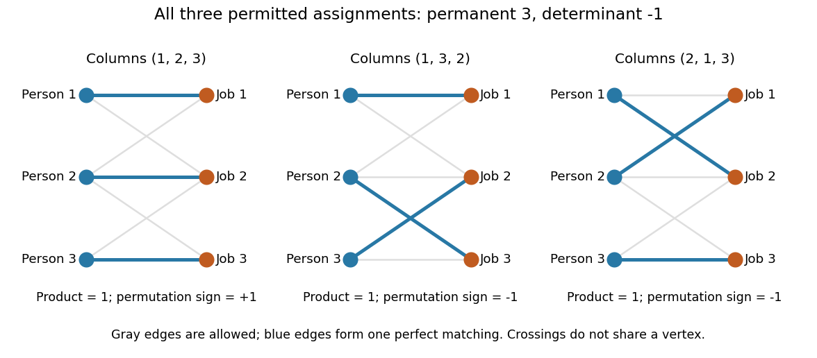
Three allowed one-to-one assignments contribute positively to the permanent, while their permutation signs give a determinant of minus one
. Details. 
A zero determinant need not mean that no assignment exists. The two-by-two all-ones matrix has permanent and determinant : its two assignments cancel in the determinant. The nonzero determinant criterion for a perfect matching is sufficient for existence, but the converse fails for a fixed zero-one matrix.
For nonnegative entries, the permanent instead sums assignment weights, with each assignment weighted by the product of its selected entries. It is then a total weight rather than necessarily an integer count. With arbitrary entries in the real numbers or complex numbers, even the permanent can have cancellation; the counting interpretation specifically uses zero-one entries. The permanent as probability of distinct independent choices gives another useful nonnegative interpretation.
There are terms in the defining sum, linking direct evaluation to the factorial. For the all-ones matrix, every term is one and the permanent is exactly ; the identity matrix has permanent one. Finding one allowed assignment and counting all allowed assignments are different questions. Their relationship to computational complexity theory was studied in L. G. Valiant, The complexity of computing the permanent, Theoretical Computer Science 8(2), 189–201, 1979. The elementary sum is useful for small examples, while the existing dense permanent approximation describes a more specialized way of estimating large counts.
A rank-one matrix update changes a matrix by an outer product . For real vectors , its action on an input vector isThe dot product reads one scalar from the input, and the correction moves the output along . All correction outputs therefore lie in one linear span. If either vector is zero, the update is zero; otherwise the correction is a rank-one matrix. The full updated matrix need not have rank one.
For example, chooseThe update sends to the correction . Although all four entries change, there is only one direction of correction. Adding it to the identity matrix gives .
This special structure allows existing work to be reused. The matrix determinant lemma updates the determinant using one scalar, and the Sherman–Morrison formula updates the matrix inverse using an outer product. Such formulas are useful when a linear system changes slightly after a new observation or a parameter adjustment: the unchanged part can retain its LU decomposition. The term rank-one describes the rank of the correction, not the size of the entry changes. [ref]
https://ocw.mit.edu/courses/18-065-matrix-methods-in-data-analysis-signal-processing-and-machine-learning-spring-2018/988b4c05680f40a5a4b3be7004a32500_XhSk_Lw2X_U.pdf. Gilbert Strang, MIT 18.065, Lecture 14: Low Rank Changes in A and Its Inverse
.A low-rank approximation replaces an matrix by a matrix of matrix rank at most a chosen integer , with , while making an explicitly chosen error norm small. The point is to describe many entries using a few shared patterns: an image compression may retain broad brightness patterns while discarding finer ones. The approximation is useful when the saved storage or computation justifies the lost detail. A small matrix rank alone says nothing about the error.
The compact representation is a sum of outer products, equivalently a product of two thin matrices:Here are the columns of , and the star denotes the conjugate transpose; over the real numbers use the transpose. The rank bound for a matrix product gives . Conversely, choose a basis of the column space of as the columns of , and put the coordinates of each column of into ; pad with zero columns if the matrix rank is smaller than . Each nonzero outer product is a rank-one matrix: it repeats a single column pattern at different strengths across the columns.
Keeping the two factors stores scalars instead of . This saves space only when . The usual singular value decomposition representation stores scalars because it keeps the singular values separately; absorbing them into one factor removes that extra array. These are representation sizes at equal scalar precision, before file overhead. See Uschmajew and Vandereycken, §9.2: thin factors and their storage, and Illinois CS 357, Low-rank approximation: storing singular vectors and values.
The factors also give without forming the full matrix . Direct evaluation uses scalar multiplications, compared with for a dense matrix applied to a vector. For , the two factors contain scalars rather than , and the same counts describe these multiplication costs. Constructing the factors is a separate cost. Moreover, a low-rank approximation need not be a sparse matrix: the constant matrix whose entries are all has matrix rank despite having no zero entries.
For the standard unweighted problem, write a singular value decomposition with and singular values . Retain the first paired left singular vectors and right singular vectors:The Eckart-Young-Mirsky theorem says that this same minimizes both of the following error norms over all matrices with matrix rank at most :where and an empty sum is zero. Here the Frobenius norm is , whereas the operator norm is specifically induced by the Euclidean norm, . The first aggregates errors in all entries; the second bounds the worst output error for a unit vector input. These formulas apply to real and complex matrices. [ref]
https://math.uchicago.edu/~may/REU2016/REUPapers/Mazeika.pdf. Mazeika, §§4.1 and 4.3: norms and optimal singular-value truncation
For , a relative Frobenius norm tolerance is met precisely when the discarded squared singular values sum to at most . Thus one can choose the smallest suitable before reconstructing the matrix. Many individually small discarded singular values can still have a large combined error. An operator norm tolerance instead tests only the largest discarded singular value, . The two questions can therefore select different ranks.
The following stipulated matrix makes the tradeoff visible. Define four real vectors of length :The vectors are orthonormal, so this is already a singular value decomposition written as outer products, with positive singular values . All entries lie between and and can be displayed as brightnesses. The first component is uniform brightness, the second distinguishes broad blocks, and the last two supply finer alternating patterns. This is a designed arithmetic example, not measured image data.
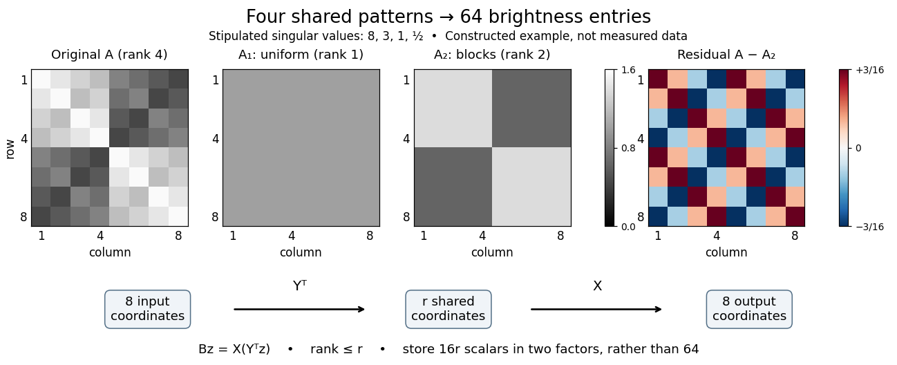

Here has every entry equal to , while has entries within the two diagonal blocks and in the other two blocks. For instance, becomes : its error is . The full residual is , whose Frobenius norm is and whose operator norm is . Since , the relative Frobenius norm error is . Two thin factors use scalars, or if the normalized left singular vectors, right singular vectors, and singular values are stored separately, instead of dense entries.
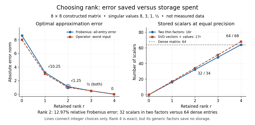

Retaining three components reduces the Frobenius norm error to while using scalars in two factors. Retaining all four reconstructs exactly but uses scalars, giving no saving in this generic representation; keeping the singular values separately uses . Our particular sign patterns could be encoded more economically, but that would exploit an additional structure beyond the general low-rank approximation. The striking feature is that numerical error and storage can both be read from the decomposition, rather than judged only by how smooth the picture looks.
The constraint is deliberately matrix rank at most . The truncation has . If , the best approximation is itself, with zero error. Requiring matrix rank exactly can destroy attainment: for and , the matrices have matrix rank for , and both error norms equal . Their error has infimum zero, but no rank-two matrix attains it. If , the displayed does have matrix rank exactly and attains the same minimum under either constraint.
Optimality also does not always mean uniqueness. For , the best Frobenius norm approximation is unique when . [ref]
https://link.springer.com/chapter/10.1007/978-3-030-31351-7_9. Uschmajew and Vandereycken, Theorem 9.1: uniqueness across a singular-value gap
A positive tie across the cutoff permits different choices: for and , both and have Frobenius norm error and operator norm error . More generally, is optimal for every real unit vector in the first two coordinate directions. Rotating which tied direction is kept changes the approximation. Repeated singular values entirely inside the retained group do not change its sum of outer products. At the only feasible matrix is zero; at the unique zero-error approximation is , even if some singular values are tied at zero.A strict gap does not guarantee uniqueness for the operator norm. For and , every with has matrix rank and error , which is optimal. Only minimizes the Frobenius norm, since . An unchanged worst direction can hide extra error in another direction under the operator norm.
Finally, these guarantees concern the stated norms and the sole matrix rank constraint. They do not establish that a discarded pattern is noise or irrelevant to a particular task: the finer patterns in our constructed example were put there intentionally. Adding entrywise weights or restrictions on the factors changes the problem, so the Eckart-Young-Mirsky theorem above does not automatically solve it. For historical context, the original 1936 matrix problem is documented in the existing Eckart-Young-Mirsky theorem section.
Two vectors spanning a hyperbolic plane. For an alternating bilinear form, choose ; then their span is nondegenerate. For a quadratic form with polar form , require also . The analogous definition for a Hermitian form uses two isotropic vectors of pairing one. Extending such pairs to adapted bases is useful for constructing form-preserving maps.
An aperture in a rigid plane with prescribed harmonic normal displacement radiates into a half-space. Superposing acoustic monopoles, each doubled by its same-sign rigid-wall image, gives the stated integral, where is the distance from aperture element to observer. In the acoustic far field, expanding to first order across the aperture identifies the angular radiation amplitude with the aperture's Fourier transform.
Linearizing inviscid barotropic flow about uniform rest gives , not automatically . Irrotational linear acoustics therefore requires zero initial vorticity or restriction to the longitudinal acoustic mode. A time-independent divergence-free field, with zero pressure and density perturbations, is a nonacoustic solution of the linearized equations.
There are unlisted articles, also show them or only show them.