A Laurent coefficient is a coefficient in the Laurent series of a holomorphic function on an annulus. Integration around a circle in the annulus gives the displayed formula, including negative indices. The coefficient is the residue.
A Born-Haber cycle uses Hess's law to infer a lattice energy from measurable enthalpy differences and isolated-species data. The motivating difficulty is that separating a mole of an ionic crystal into mutually separated gaseous ions is not a convenient direct calorimetry experiment. Instead, compare two accounting routes between the same elemental reference states and the same solid. Because enthalpy is a state function, the signed differences close exactly when all inputs describe compatible states. These routes do not assert a reaction mechanism or a temporal sequence of reaction intermediates.[ref]
For one mole of sodium chloride formula units, the overall formation reaction isThe stoichiometry requires half a mole of diatomic chlorine molecules, supplying one mole of chlorine chemical atoms. A half coefficient counts an amount of substance; it does not describe half of an individual molecule. Write each auxiliary chemical reaction with its own sign:Here is the sublimation enthalpy, the enthalpy of atomization of chlorine per mole of chemical atoms, and the molar ionization enthalpy represented by the ionization energy input in elementary treatments. If the bond-dissociation energy table gives the compatible molar enthalpy for , use half that number for . Both ions in the last step are gaseous, and no aqueous hydration of ions belongs in that step.
Adding these equations cancels the gaseous chemical atoms, the gaseous ions and the free electron, leaving precisely the overall formation reaction. ThusThe closed traversal returns from the solid to the elemental reference states, adding ; therefore . Notice that the signed attachment term is negative. Substituting a positive spectroscopic electron affinity for would reverse the attachment contribution.
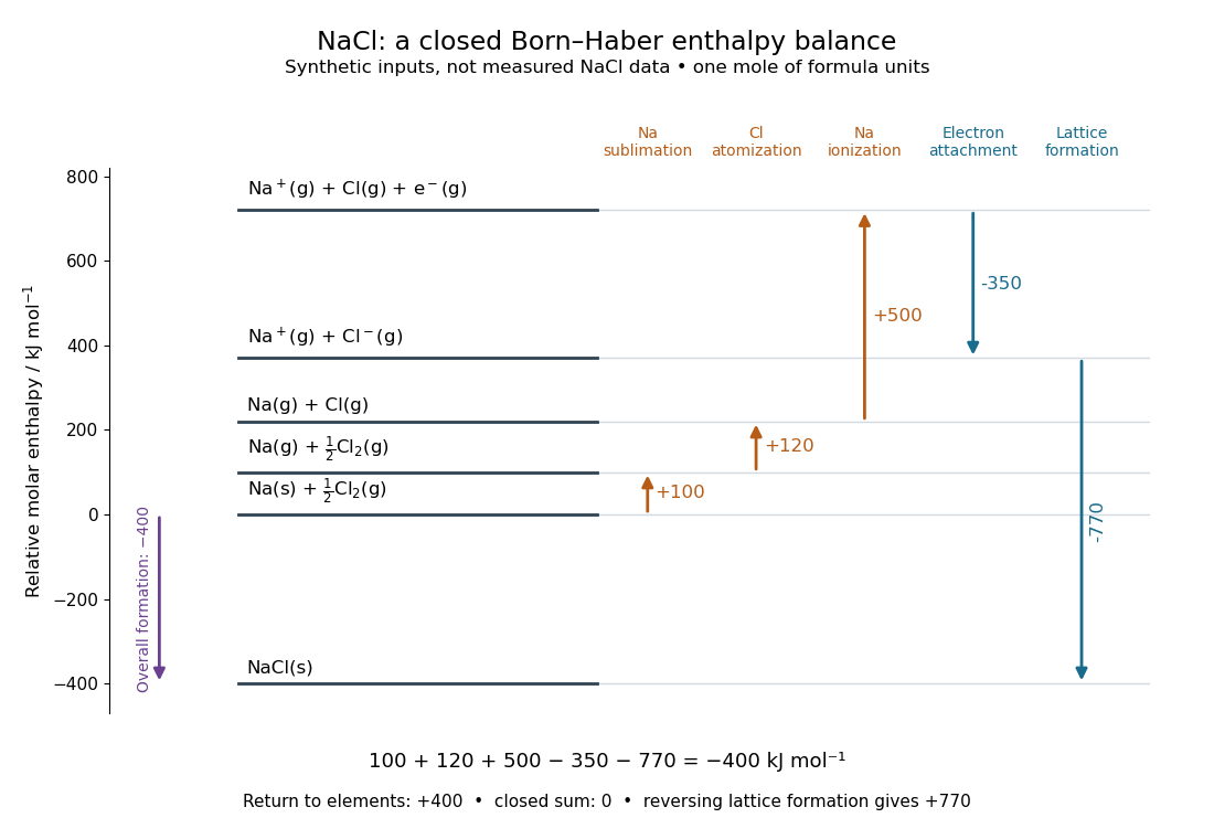
A closed Born-Haber cycle for sodium chloride using explicitly synthetic molar enthalpies: levels represent complete material inventories, and horizontal position is bookkeeping rather than a reaction coordinate
. Details. 
The diagram deliberately uses invented, internally consistent inputs in : , , , and . Preparation of separated gaseous ions raises the enthalpy by , so and . The closure check is . These numbers are not measured sodium chloride data and do not replace the source's example in lattice energy. Every level retains one sodium nucleus, one chlorine nucleus and zero total electric charge; the ionization level explicitly retains the free electron.
Ice-melting calorimetry measures the fusion enthalpy through conservation of energy, rather than inferring it from the small temperature change of the melting ice itself. In a mixing experiment, warm water and the container cool while added ice melts and the resulting water warms. Their combined energy balance separates fusion from sensible heat.
Weigh the container and stirrer, then weigh the added warm water to obtain . Let the container and water reach a common initial temperature . Prepare ice in a clean ice-water mixture near , rather than assuming freezer ice is already at ; drain and blot its surface immediately before transfer. Add it without splashing, stir gently, and record temperature before addition and until after the last ice disappears. Reweigh to find the added mass . Wisconsin's laboratory guide specifies drying each piece, weighing before and after, and recording the temperature history; it places the initial and final temperatures on opposite sides of the jacket temperature to reduce net environmental exchange. [ref]
https://badger.physics.wisc.edu/trash/lab_old/manual/node30.html. University of Wisconsin, H-2: Latent heat of fusion of ice, procedure
For fully melted, initially dry ice at , a common final temperature , constant water specific heat capacity at constant pressure , and apparatus heat capacity initially at ,Here denotes net heat entering the apparatus from its surroundings. The left side supplies the fusion enthalpy and the sensible heat on the right; the water produced by melting must be warmed too. The balance extends Case Western's mixing demonstration by including the apparatus and environmental terms. If the specific heat capacities vary appreciably, replace their products with the corresponding temperature integrals. [ref]
https://case.edu/artsci/phys/courses/demos/spec.htm. Case Western, mixing-calorimetry energy balance
Determine independently, for example by a warm/cold water mixing balance with no phase transition, including the wetted stirrer and thermometer in the apparatus. Check the thermometer calibration, keep the lid in place between transfers, and monitor the surroundings. Before/after drift and a comparable run without ice help bound ; such corrections assume comparable heat transfer conditions and are not automatically exact. Choosing a jacket temperature between and reduces exchange but does not prove . Ensure all the ice has melted and the contents are well mixed before using the measured : with residual ice, the weighed addition is not the mass that has undergone fusion. Repeat the experiment and report measurement errors in mass, temperature, and the leak correction.
An independent way to see the plateau is David Roundy's Oregon State experiment: heat an ice-water mixture slowly with a waterproof resistor in an insulated cup, stir, and record temperature, heater electric current , electric potential difference and elapsed time. Plot temperature against , recording changes in or . The initial solid mass must exclude accompanying water. For a boundary enclosing the heater as well as the sample, this input is electrical work, so under the constant-pressure assumptions above. Across an ideal isothermal plateau the apparatus has no sensible heat change, giving ; departures from uniform temperature require accounting for the heater and container response. [ref]
https://paradigms.physics.oregonstate.edu/act/handout/2108. David Roundy, Oregon State, Ice Calorimetry Lab: apparatus, stirring and electrical input
Optical gain is amplification of light by a medium. Here the small-signal intensity gain coefficient has units : for fixed populations, a weak beam obeysin the nondegenerate resonant two-level model, with common transition cross-section . Thus includes the competition between stimulated emission and photon absorption on that transition. Separate passive intensity loss gives . Both coefficients describe light intensity, not wave amplitude; the corresponding field-amplitude exponent is half as large. [ref]
https://ocw.mit.edu/courses/6-974-fundamentals-of-photonics-quantum-electronics-spring-2006/2641db6431ea70989c29e8512d5d91a7_chapter6.pdf. Franz Kärtner, MIT 6.974, §§6.7–6.8: amplification and stimulated-transition cross-section
.For , and , the single-pass intensity multiplier is . This is amplification during one passage, before mirror losses. Population inversion can therefore yield positive optical gain while the complete oscillator remains below laser threshold.
Stimulated emission is emission induced by incident light, in contrast with the unprompted decay in spontaneous emission. It supplies the amplification mechanism of a laser. [ref].
For an emitter with upper and lower energy values , the resonant photon has frequency satisfyingwhere is the Planck constant. In the elementary photon picture, an incident photon stimulates an emitter in the upper quantum state to emit an additional photon into the same optical normal mode, with the same frequency, propagation direction and photon polarization. The emitter supplies the extra energy; the stimulating photon is not consumed. This builds the existing field and its optical coherence. An emitter in the lower quantum state can instead undergo photon absorption, so stimulated emission alone does not establish net optical gain.
For example, a gap corresponds to and a vacuum wavelength of about . One ideal stimulated emission event converts one incoming photon into two outgoing photons in the selected optical normal mode, adding of light energy while lowering the emitter's energy by that amount.
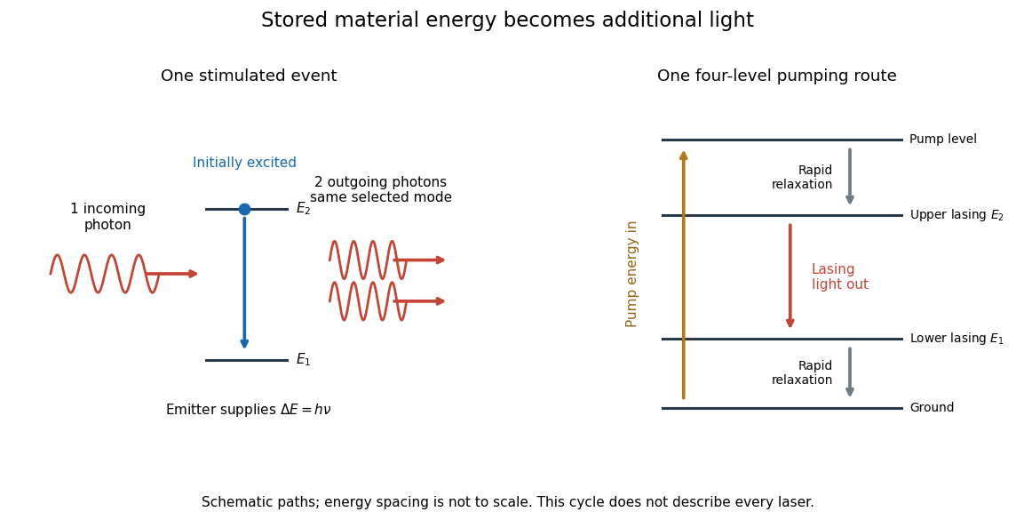
Stimulated emission and one illustrative four-level laser pumping cycle
. Left: one incoming photon induces an additional photon while the emitter falls from to . Right: pumping supplies energy, rapid relaxation feeds the upper lasing state, stimulated emission supplies light, and rapid lower-state relaxation completes a four-level cycle. These paths are schematic, not universal to all lasers; line spacing is not to scale. Details.
A galaxy survey measures positions and other properties of a selected galaxy sample. A spectroscopic survey uses cosmological redshift to estimate radial distance, with corrections for peculiar velocity. Its volume, selection, galaxy bias, and sampling determine which matter power spectrum modes can be inferred.
A galaxy cluster is a gravitationally bound collection of galaxies, diffuse gas and dark matter. Much of its ordinary matter can reside in hot intracluster gas, visible through thermal bremsstrahlung and the Sunyaev-Zeldovich effect. The two signals weight the electron density differently, making the cluster useful both as a structure-formation probe and, with a geometrical model, as a distance indicator.
The cosmological two-point correlation function measures excess pairing or correlated density fluctuations at a separation. For a statistically homogeneous and isotropic mean-zero density contrast, . For distinct points in a discrete galaxy population it instead specifies the factorial pair density, . The latter excludes self-pairs; an unsmoothed discrete-density covariance also contains a Dirac delta at zero separation. These definitions connect large-scale galaxy clustering with the matter power spectrum while keeping galaxy power spectrum shot noise separate.
For , the vector potential is a Landau gauge. Translation invariance in turns the transverse Hamiltonian into a family of harmonic oscillators in whose centres are labelled by the conserved -momentum.
Ground-state filling of two spin-degenerate Landau levels by  Codex 0 Created 2026-10-14 Updated 2026-11-05
For noninteracting electrons in a planar sample of area , neglecting Zeeman splitting leaves two spin states for each orbital. Each Landau level therefore holds electrons. When , fill the lowest level with electrons and the next with ; summing their energies gives the displayed concave quadratic in . The energies at the two integer-filling endpoints are equal.
In his 1883 paper, Osborne Reynolds investigated how the character of pipe flow depends jointly on velocity, pipe diameter and viscosity. His final dye apparatus drew water from a large glass tank through a horizontal glass tube with a smooth trumpet-shaped entrance. A separate reservoir supplied strongly colored water just upstream of the entrance; a valve below the tank controlled the outflow. The glass tube was immersed in the tank, so its internal dye band could be watched. Reynolds repeated the trials with different tube diameters and water temperatures. [ref]
https://archive.org/stream/philtrans06508925/06508925_djvu.txt. Osborne Reynolds (1883), sections 11 and 21–22, pp. 941–943 and 951–953
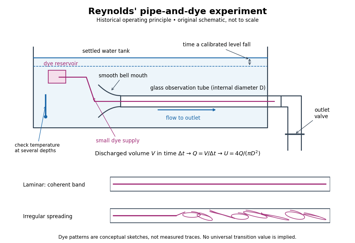
Reynolds' pipe-and-dye experiment: observe the dye while measuring discharge and temperature
. Original schematic of the historical operating principle, not a scale reconstruction. A falling tank level determines discharged volume; timing it gives flow rate. The lower dye patterns are conceptual sketches of a coherent band and irregular spreading, not measured trajectories or concentration records. Details.
The volumetric flow rate was measured independently of the appearance of the dye. Reynolds timed a one-inch fall of the tank's water level, corresponding to a calibrated discharged volume. In modern notation, if this volume is and the elapsed time is , then and . He determined the glass tubes' internal diameters by filling them with water. For a uniform bore, a known filled length and measured water volume determine ; checking bore uniformity matters because the same volume would only give an average cross-section in a tapered tube. Thermometers at different tank levels checked both the temperature and its uniformity. Reynolds compared the viscosity at different temperatures using Poiseuille's results and checked his own water by separate experiments of that type. Thus the Reynolds number estimate did not come from judging the dye band or from assuming that transition occurred at a preset value. [ref]
https://archive.org/stream/philtrans06508925/06508925_djvu.txt. Osborne Reynolds (1883), sections 21–22 and the reductions following Table I, pp. 951–955
A practical repetition can instead collect a known outflow volume in a measuring vessel and time its collection, or weigh the collected water and divide its mass by mass density. Measure the internal diameter, rather than the external diameter, and obtain kinematic viscosity at the measured water temperature from independently established properties or a separate viscosity measurement. Record the dye appearance and observation position alongside , , temperature and the resulting Reynolds number. These are alternative measurement procedures following , not additional historical claims about Reynolds' dye apparatus.
Begin with settled water and a small dye supply, then open the outlet valve in small steps. Reynolds saw a thin straight band at sufficiently low speeds. With a tank that had not fully settled, the band could wander while retaining its coherence. At higher discharge it could abruptly spread into the surrounding water downstream of the entrance. Short illumination by an electric spark resolved curls within what otherwise looked like a colored cloud. This connected the visible breakup with internal irregular motion rather than merely the appearance of an opaque pipe. [ref]
https://archive.org/stream/philtrans06508925/06508925_djvu.txt. Osborne Reynolds (1883), sections 11 and 22, pp. 942 and 951–952
The controls are part of the result. Reynolds used a smooth entrance and let the tank rest to reduce inlet disturbances. He found that a heated tank could retain slow circulation as it cooled, so measuring one temperature was insufficient: thermal uniformity and residual motion also mattered. His wire-coil trial broke up the band below the previous onset speed, but he explicitly cautioned that once the dye was mixed he could not tell from that dye alone whether the motion became orderly again farther along the tube. In a repetition, keep the dye supply small enough to act approximately as a passive scalar, avoid a strong injection jet, and record the inlet condition and downstream observation distance. If also testing the Hagen-Poiseuille equation, allow the profile to develop and measure pressure drop between positions within the developed region; do not treat the entrance and outlet losses as part of its uniform pressure gradient. The dye experiment by itself does not establish fully developed flow. [ref]
https://archive.org/stream/philtrans06508925/06508925_djvu.txt. Osborne Reynolds (1883), sections 21–23 and 26, pp. 951–956 and 959
The experiment's usefulness is that it compares a visible change in the motion with independently measured scales. Repeating it with several diameters and temperatures, while controlling disturbances, tests the organizing role of the Reynolds number. Its limitations are equally instructive: dye is a tracer of transport, diffusion still acts in laminar flow, and a local dye observation cannot by itself prove that turbulence persists throughout an arbitrarily long pipe.
A regular Lagrangian defines a fibre derivative and the Cartan one-form . Its two-form is nondegenerate when the velocity Hessian is invertible. The energy is . The equation determines the Euler–Lagrange vector field. A hyperregular Lagrangian makes the fibre derivative a global diffeomorphism and transports this dynamics to Hamiltonian phase space.
For a finite constrained optimum value and optimization Lagrangian , the strong Lagrangian property means that some finite Lagrange multiplier attains the dual lower bound exactly: . It includes dual attainment, but need not include primal attainment. It is equivalent to a non-vertical supporting hyperplane of a value function: a supporting slope gives , hence ; weak duality gives the opposite inequality. Conversely the infimum identity bounds every below by ; taking the infimum over gives the supporting inequality. No convexity assumption is needed for this equivalence.
The Lagrangian perturbation compares a variable on the same moving fluid element before and after a displacement. Taylor expansion of the background value at the displaced position gives the displayed relation to an Eulerian perturbation. For an adiabatic ideal gas, even when the equilibrium entropy varies spatially.
The Eulerian perturbation compares field values at the same spatial location, rather than following a fluid element. To first order it satisfies . Thus a field advected unchanged by individual elements can still have a nonzero Eulerian perturbation in an inhomogeneous background.
For real not all equal, let , and . The unique minimizer of under , is , with minimum . To prove sufficiency, the optimization Lagrangian with multipliers , is a sum of squares in plus a constant. Equivalently every feasible satisfies .
For a smooth constrained maximum subject to , suppose smooth optimizers and multipliers satisfy . Differentiating the constraint gives , and the chain rule gives . Thus a Lagrange multiplier measures the marginal value of relaxing its corresponding constraint. A global supporting Lagrangian duality representation implies the needed stationarity, but local stationarity and smoothness alone suffice for this derivative identity.
For radius and height , volume is and area including both ends is . The Lagrange multiplier equations give . Substituting the constraint gives the one-variable function , which tends to infinity at both ends and has its only stationary point at . This proves the stationary cylinder is the unique global minimizer.
For an axis-aligned box, maximize subject to . The Lagrange multiplier equations imply . Boundary boxes have zero volume, so this gives the maximum. Arbitrary orientation cannot improve it: averaging the ellipsoid inequality over the eight vertices gives a sum of three squared transformed half-edge lengths at most one; the determinant bound and arithmetic-geometric mean bound their product by .
This nonlinear dispersive equation replaces the quadratic KdV nonlinearity by a cubic one. In the displayed sign convention, the Miura transformation maps its solutions to . Its scaling symmetry is .
There are unlisted articles, also show them or only show them.