A type-IIB D-brane with seven spatial dimensions. Its RR charge is magnetic with respect to , or electric with respect to the dual eight-form potential. Its transverse geometry is codimension two, so the simple asymptotically flat harmonic formula for lower-dimensional D-branes does not apply unchanged.
A type-IIB D-brane with five spatial dimensions. Its RR charge is magnetic with respect to the two-form potential , or electric with respect to the dual six-form potential. It is distinct from the NS5-brane, whose charge is magnetic under the NS-NS two-form and whose string-frame tension has a different power of the coupling.
A standard positive-total form of the Dvoretzky-Motzkin cycle lemma uses a nonempty sequence of integers satisfyingExactly starting positions have every nonempty partial sum strictly positive, using the same rotation convention as the sum-one cycle lemma. Negative entries can be arbitrarily large in magnitude, and zero entries are allowed. Addario-Berry's proposition 2.2.1 gives an equivalent form with increments at least and negative total; reversing the sequence and changing all signs gives the form here. [ref]
https://problab.ca/louigi/notes/ssprob2021.pdf#page=39. Addario-Berry, Lecture notes: 2021 CRM-PIMS Probability Summer School, proposition 2.2.1, p. 39
Four starts, two successes. For , the sum is . Starts and give partial sums and , respectively. Start gives and touches zero; start gives and begins below zero. Thus exactly two starts are good. The rotated sequence has the same positive total, but its first start is bad: a positive final lead alone does not control earlier partial sums.
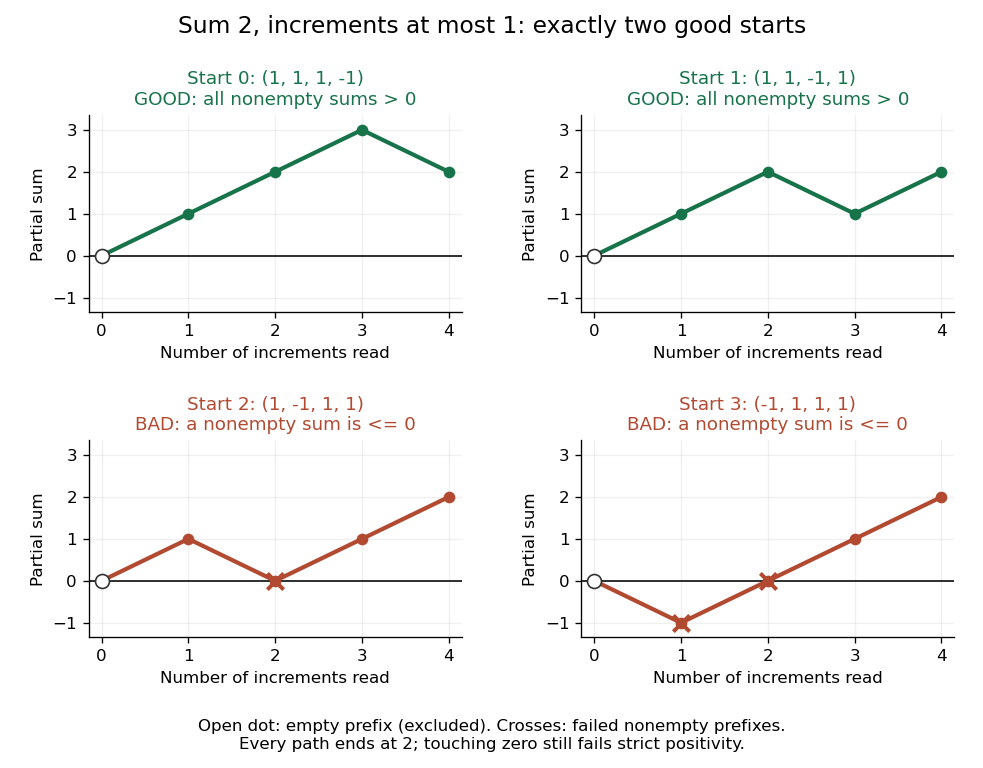
All four starts of : the cycle lemma with increments at most one counts precisely the two paths whose nonempty partial sums stay strictly above zero
. Details. 
Positions can give identical words. The sequence repeats a block of length three and has sum two. Its good starts are and , both giving the same word with partial sums . Starts and touch zero; starts and begin negatively. The cycle lemma with increments at most one counts two starting positions even though there is only one distinct good rotated word. Counting distinct words would lose the multiplicity that makes the statement true.
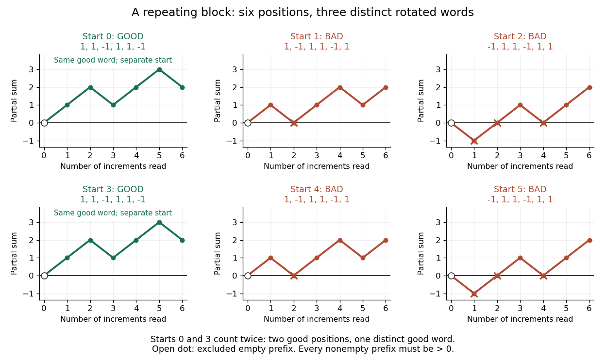
Six starting positions of the repeating sequence : starts and produce identical good words and count twice
. Details. 
The upper bound matters. The one-entry sequence has positive integer sum two, but only one starting position. Thus the sum- conclusion fails for arbitrary positive increments when . The sum-one cycle lemma above needs no such upper bound. Strict positivity also matters: counting paths that merely stay at or above zero would include additional starts in both diagrams.
From rotation to enumeration. For a fixed admissible sequence, a start chosen from a uniform distribution on a finite set of its positions is good with probability . More generally, let be any finite set of length- sequences satisfying the increment bound and total , closed under rotation. Double counting pairs consisting of a sequence and a good starting position givesFor each good output sequence and each of the positions, inverse rotation gives one such pair, even when several rotated words coincide. For example, the four sequences containing three votes and one vote have exactly vote orders with a strictly positive running lead: and . This is how the cycle lemma with increments at most one converts many prefix inequalities into a simple counting factor.
Model a spatially uniform cell membrane as a capacitor of membrane capacitance in parallel with membrane electrical resistance and a fixed leak reversal potential . Exclude active ion channels, seal leak current and pipette capacitance. For electric current injected into the biological cell, electric charge conservation yieldsStarting at and applying constant gives the ordinary differential equation solutionThe steady state rise is ; the time constant is . With , , and , the rise is and . At one time constant the rise is . The figure's uncompensated pipette voltage adds for . The membrane voltage is continuous at step onset in this model, while the pipette voltage immediately acquires that access drop.
Checking the units is instructive: electrical resistance times capacitance has units , and electric current times electrical resistance has units of voltage. Unlike the passive voltage clamp transient under patch-clamp series resistance, this ideal current clamp membrane time constant is set by , not . Strong current steps can recruit voltage-gated ion channels; the passive model then fails and cannot generate an action potential. Small pulses of both signs, stable access and repeated baseline measurements help test whether the passive approximation is appropriate.
A saddle point of a scalar function is a stationary point with nearby values both greater and less than its value. An indefinite Hessian matrix proves this by choosing directions with opposite signs of the quadratic term. A degenerate Hessian matrix may require higher-order terms: has a saddle point of a scalar function at the origin despite a zero quadratic coefficient in the direction. This is distinct from a saddle equilibrium of a dynamical system.
For , the origin is a strict local minimum. The four axis points at distance one have Hessian eigenvalues and . The four diagonal points with have Hessian eigenvalues and . Thus for the diagonal points are the global maxima and the axis points are saddle points of a scalar function; for these roles reverse. In polar coordinates, , where . Maximizing over gives and proves the global statements. At , , so the entire unit circle is the maximum set.
For with , its stationary points are the origin and, when , , . The origin is a strict local minimum for and a saddle point of a scalar function for . At its Hessian matrix is singular, but the vertical line gives positive values and the parabola negative values, so it remains a degenerate saddle. The other stationary points have Hessian determinant and are saddles.
In the analysis of a phase transition, a critical dimension is a spatial dimension at which the character of fluctuations and critical behavior changes. Below a lower critical dimension the relevant ordered phase cannot persist; above an upper critical dimension mean-field critical exponents apply. This is distinct from the critical dimension of string theory, where cancellation of quantum anomalies selects a target-spacetime dimension.
Universality of critical phenomena is the agreement of critical exponents or normalized scaling forms between microscopically different systems. Dimension, symmetry and interaction range help determine the universality class. A renormalization-group flow can explain this agreement by showing that different microscopic models approach the same fixed-point description, while irrelevant differences fade at large scales.
A simple symmetric random walk on a cycle of vertices, started at vertex zero, has its last newly visited vertex uniformly distributed on the other vertices. To prove this for a specified vertex , cut the cycle at , representing it by a path with absorbing endpoints both corresponding to . All other vertices are visited before exactly when both interior endpoints are visited before absorption. After the first hit on either interior endpoint, the probability of reaching the other before the adjacent absorbing endpoint is by gambler's ruin. The Strong Markov property makes this the desired probability, independent of the original start position. For the sole unvisited vertex has probability one.
Suppose a finite-alphabet transition kernel is uniformly positive and histories agreeing in their most recent symbols have total variation distance at most . Choose decreasing bounds with and summable tail. A maximal coupling can be dominated by a match-length chain that increments with probability and resets with probability . Its chance of never resetting is . Successive failed attempts therefore end almost surely, leaving a final infinite run of matches. The dominating chain does not depend on the histories, so future-block laws forget the remote past uniformly. This proves uniqueness of a two-sided law with the prescribed transition kernel without assuming stationarity first.
Cosmological background intensity from comoving emissivity by  Codex 0 Created 2026-10-14 Updated 2026-11-05
Let be the comoving spectral emissivity, namely total emitted spectral luminosity per comoving volume. In a homogeneous transparent FRW metric, a radial shell contributes its comoving volume times the cosmological spectral flux-density relation. Its transverse-area factors cancel, leaving the displayed integral. In a flat model this cancellation is explicit: , whereas . Absorption inserts a transmission factor, and evolving sources are represented by the redshift dependence of .
Cosmological bolometric background from conserved sources by Codex 0 Created 2026-10-14 Updated 2026-11-05
Codex 0 Created 2026-10-14 Updated 2026-11-05Normalize the scale factor to . Identical isotropic sources of bolometric luminosity and conserved comoving number density produce all-sky radiative flux in a transparent FLRW metric. The source counts on an FLRW past light cone and cosmological flux dimming cancel the transverse shell-area factor. For arbitrary proper source density the expression is instead . The intensity per solid angle is . A detector of collecting area receives power under an all-sky effective-area convention.
Our observer location is not specially privileged. In cosmology this assumption allows cosmological isotropy observed around us to be interpreted statistically as cosmological isotropy around other typical observers. It is an assumption about typicality, not a deduction from one observer's sky or from the Einstein field equations alone.
Cosmological isotropy means that coarse-grained spatial observations or their statistics are unchanged by rotations about an observer. In an FRW metric it holds about every comoving location. cosmological isotropy about a single location is weaker than spatial homogeneity: a radially inhomogeneous model centred on that location can also have an isotropic sky.
In a radiation-dominated toy model with , setting the interaction rate equal to the Hubble parameter gives the displayed decoupling scale. The transition defines . For smaller masses, . An instantaneous chemically equilibrated cosmological particle freeze-out estimate gives . This estimate presupposes number-changing thermal equilibrium, radiation domination and the assumed rate law, rather than following from elastic thermalization alone.
A rate proportional to competes with radiation-era expansion proportional to . The interaction-to-expansion ratio therefore grows as the universe cools, crossing unity near . If a phase transition occurs at , this high-temperature interaction never establishes thermal equilibrium before the transition. Subsequent faster number-changing processes may still establish a thermal distribution; the initial state is not automatically Fermi-Dirac just because the particles are relativistic.
A thermal relic is a surviving particle population whose earlier abundance was set by chemical thermal equilibrium with the cosmic plasma. After number-changing reactions cease and cosmic entropy is conserved, its comoving abundance is described by the yield . A relativistically decoupled species can retain an appreciable yield, whereas a species remaining in thermal equilibrium after becoming nonrelativistic is subject to Boltzmann suppression. Its later mass density, lifetime and momentum distribution determine its cosmological effects.
There are unlisted articles, also show them or only show them.