A direction field for places a short segment with slope at each sampled point where is defined. A function graph of a solution of a differential equation follows these segments: its tangent line has exactly the prescribed slope. Segment length is a drawing choice, rather than a speed; arrows, if used, point toward increasing . An isocline collects points with one common slope.
For Newton's law of cooling, with time in minutes and temperature in degrees Celsius, the slopes at are respectively degrees Celsius per minute. Each horizontal row is an isocline, because this autonomous differential equation has no explicit time dependence. Above the solutions of a differential equation descend, below they rise, and is an equilibrium point.
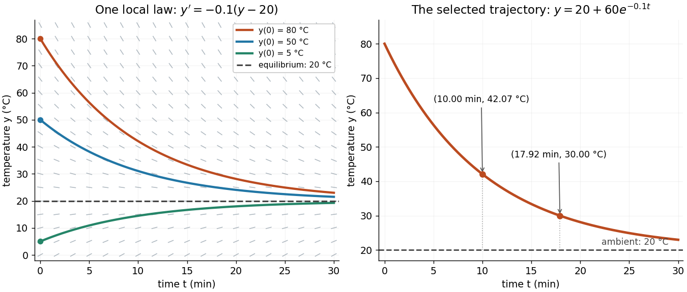

The highlighted initial condition selects one curve from the family. The picture reveals approach to the equilibrium point before any algebra is done. Under the hypotheses of the Picard-Lindelöf theorem, distinct function graphs of solutions cannot cross or even meet in the time-state plane. A direction field alone does not guarantee uniqueness: several curves can share a tangent line at the same point when those hypotheses fail. See the delayed-start example under initial value problem.
This geometric interpretation is developed in Direction Fields, Isoclines, Integral Curves.
Smoothness describes the degree of differentiability of a function. The class has continuous derivatives through order ; a smooth function is of class .
If a real function has a finite derivative at , its difference quotient tends to and is bounded for sufficiently small nonzero increments. Multiplying it by the increment shows , proving continuity at . The converse fails: the absolute value function is continuous but not differentiable at zero.
If , and both endpoints tend to , differentiability gives with . The error in the secant is bounded by for large . Thus these secants converge even when either endpoint equals .
A function with and the displayed bound has zero Fréchet derivative at zero, since . In particular, a bounded oscillatory factor multiplied by a quadratic expression is differentiable at the origin even if the oscillations have no limit themselves. For , extended by zero on the two diagonal lines, this damping works at the origin. At a nonzero point of either line, the quadratic factor instead vanishes to first order along a transverse direction; the difference quotient oscillates without a limit. Thus the differentiability set is the complement of those two lines together with the origin.
Differentiability does not imply continuity of the derivative by  Codex 0 Created 2026-10-14 Updated 2026-10-18
Extend the displayed function by . Its difference quotient at zero is , which tends to zero. Away from zero its derivative is . At this derivative equals , whereas at it equals . Thus differentiability implies continuity of the function but does not imply continuity of its derivative.
For a positive odd integer , Fermat's factorization method searches for integers satisfying . Start at and test successive values until is a perfect square . The difference of two squares then gives . For an even input, remove factors of two first.
The search always reaches at least the trivial factor pair , at . It is useful when a nontrivial factor pair is close: that pair is reached at , withA small difference between factor sizes therefore requires few trials. This is a different advantage from looking for a small prime factor by trial division.
Dielectronic capture is the resonant capture stage inverse to a specified autoionization channel. For an entrance ion of weight and resonance of weight and energy , its Maxwellian coefficient is . This follows by equating capture and autoionization fluxes at thermodynamic equilibrium. Capture alone need not produce a permanently recombined ion.
Radiative stabilization occurs when a photon emission from an autoionizing state leads to a bound state, preventing electron re-ejection. For one radiative channel and one autoionization channel, its probability is . With several channels, use summed losses and the total rate of successful stabilizing decays; a cascade through another autoionizing state requires its eventual survival probability.
For temperature-independent atomic rates and an isolated positive-energy resonance, dielectronic recombination has the displayed dependence. Differentiating its logarithm gives a maximum at . A sum of resonances can have several peaks, and near-threshold resonances change the low-temperature behavior. Collisional destruction of captured high levels can introduce density dependence.
A reduced biological response to insulin; it is a property of response, not simply a low insulin concentration. The glucose clamp technique helps separate these quantities.
Diabetes associated with marked loss of insulin-producing beta-cell function, commonly through autoimmune destruction. The mechanism differs from defining the disease solely by age at diagnosis.[ref]
Type 1 Diabetes Mellitus by Merck Manual Professional Edition. Definition and pathophysiology
Cell differentiation is the acquisition of a specialized cell state, involving changes in structure, function and gene expression. A neuron and a red blood cell illustrate different outcomes: signaling and oxygen transport. Different functions usually do not require a different inherited DNA sequence for each function. The shared-genome principle concerns nucleated precursors and most nucleated descendants: a mature mammalian red blood cell has lost its cell nucleus and mitochondria, so it is not an example of two mature biological cells both retaining the same nuclear DNA. [ref]
Biology 2e by Mary Ann Clark and others. Biology 2e, §40.2, Red Blood Cells: specialization and absence of a nucleus and mitochondria at mammalian maturity
The puzzle is how a shared set of genes supports different jobs. Gene expression changes which RNA and proteins a biological cell produces, and in what amounts. A transcription factor can regulate several genes; different combinations of regulators can interpret the same signal differently. Stable regulatory patterns can persist through the cell cycle, providing memory of developmental history. Specialization therefore usually changes use of inherited information, rather than replacing the genome wholesale. [ref]
Molecular Biology of the Cell, 4th edition by Bruce Alberts and others. Alberts et al., The Molecular Genetic Mechanisms That Create Specialized Cell Types, subsections The Expression of a Set of Genes Can Be Coordinated by a Single Protein and Stable Patterns of Gene Expression Can Be Transmitted to Daughter Cells, and Summary
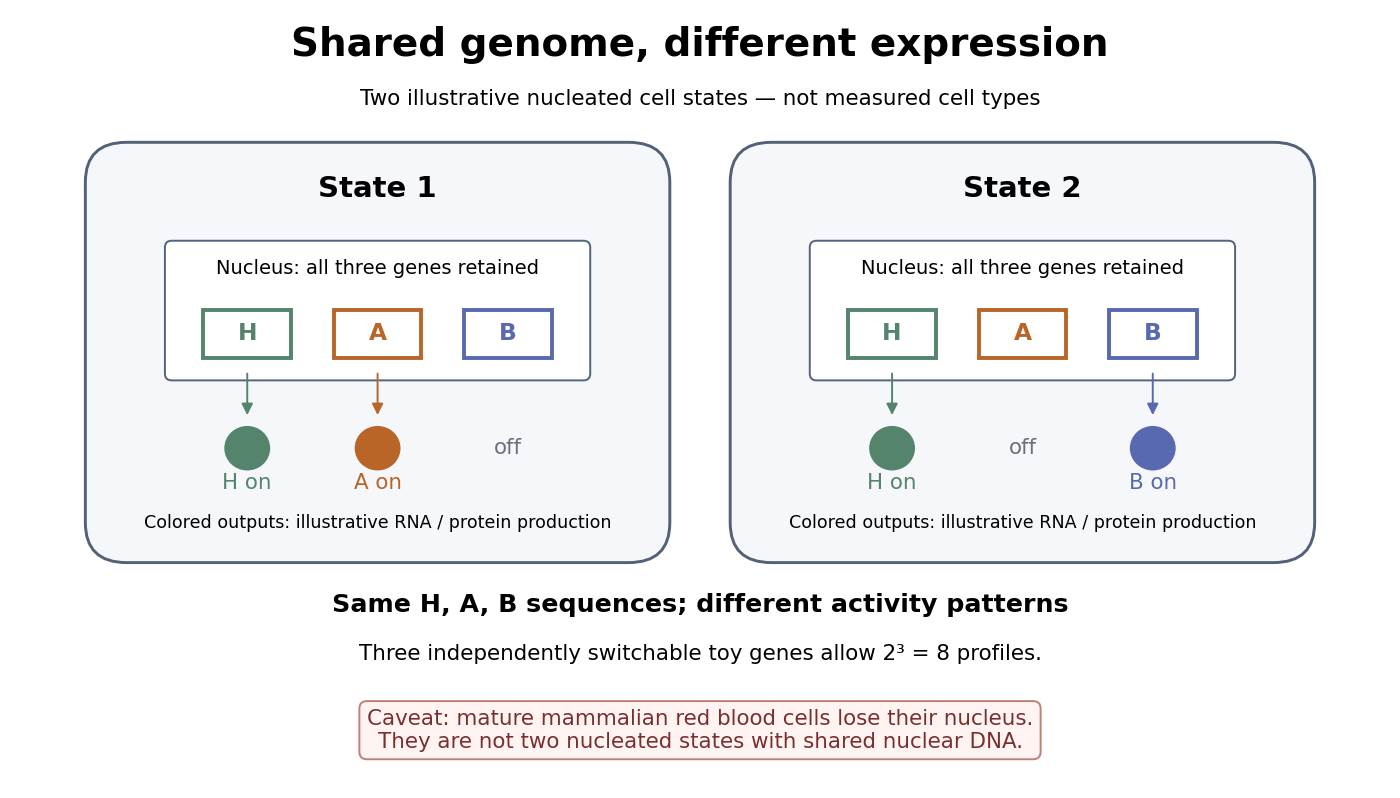

A small counting example separates sequence from activity. Suppose the same three toy genes are present in every nucleated biological cell, and independently assign each gene an on/off state. There are possible expression profiles with no DNA replacement. The figure shows only two: H and A on versus H and B on. Real gene expression is graded and coordinated, so this count illustrates possible descriptions, not a prediction of eight actual cell types. The interesting consequence is that a stable cell state can depend on how a shared record is used.
Stem cells combine self-renewal with production of differentiated descendants; progenitor cells generally have more restricted developmental options and renewal capacity. Neither term means that a biological cell must give rise to every cell type. Terminal differentiation denotes advanced specialization within a lineage, often accompanied by exit from the cell cycle. Cell fate concerns the developmental outcome of a biological cell or its descendants, whereas cell state describes its current properties. A temporary change in gene expression after signal transduction is not, by itself, proof of a new cell fate. [ref]
Anatomy and Physiology 2e by J. Gordon Betts and others. Anatomy and Physiology 2e, §3.6, Stem Cells and Differentiation: renewal, restricted differentiation potential and regulation of gene expression
The doubling map is the discrete dynamical systemon the unit circle represented by . In a binary expansion, it shifts the digits one place to the left. This makes a small uncertainty in later digits become a large uncertainty after sufficiently many iterates.
Its Devaney chaos can be checked directly. The periodic points of the doubling map are the grids ; their mesh tends to zero, giving dense periodic points. Every nonempty open arc contains an interval for large enough . Its image under covers the unit circle, proving topological mixing and hence topological transitivity. Finally, for any initial point and arbitrarily large , choose modulo one. Their initial circle metric distance tends to zero, while the distance between and is . This proves sensitive dependence on initial conditions with a fixed separation threshold smaller than .
The butterfly effect is the intuitive idea that an arbitrarily small change in an initial condition can eventually change the observed future substantially. In dynamical systems, sensitive dependence makes this precise for a map on a metric space : there is one separation scale such thatThe same works at every point, whereas and the separation time may depend on the point and the requested closeness. For a flow map, replace the iteration of a map by with some . The state space matters: restricting to a single fixed point removes the alternative nearby states needed for sensitivity.
Sensitivity is compatible with deterministic evolution. Given an exact initial condition, there is still one orbit; uncertainty concerns which exact state a measurement represents. It also allows accurate short-term prediction. For a continuous function , each fixed finite iterated function is continuous, so sufficiently close initial states remain close at any specified finite step. What fails is a single initial accuracy that controls every future step.
The logistic map illustrates both sides. At , nearby orbits in the basin of attraction of its attracting fixed point approach one another. At , arbitrarily close states can eventually separate by a macroscopic fraction of . The definition asserts the existence of separating neighbours, not that every nearby pair must separate: and have exactly the same next state under the logistic map and hence the same subsequent orbit. Nor must separation increase at every step.
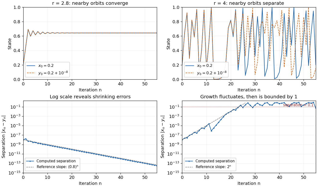
The same deterministic logistic rule can shrink or amplify initial uncertainty
. Each pair starts at and and uses the same logistic map parameter. At , the orbits approach the same attracting fixed point. At , this pair eventually gives visibly different states. The logarithmic panels expose changes hidden in the upper panels; dashed slopes illustrate the eventual contraction factor and a representative exponential growth factor . They are reference slopes, not exact formulas for these finite separations. Distances fluctuate and remain bounded by one. These computations illustrate the phenomenon; two numerical orbits alone do not establish the quantified definition. Details.
A positive Lyapunov exponent describes average exponential growth of an infinitesimal displacement along an orbit, when the relevant limit exists. It is related to sensitivity but is not a substitute for its uniform definition. For a differentiable interval map, the chain rule givesAt , the logistic map has for Lebesgue measure-almost every initial condition, while exceptional orbits can have different exponents. Finite-separation growth is only approximately exponential while the linear approximation remains useful. In a bounded state space, a separation cannot grow exponentially forever.
Sensitivity alone is also weaker than Devaney chaos, which additionally requires topological transitivity and dense periodic points. For example, on the real line has sensitive dependence and a positive Lyapunov exponent, but its only periodic point is zero, so it is not Devaney-chaotic. This distinguishes growth of uncertainty from the richer organization of recurrent orbits.
Edward N. Lorenz's "Deterministic Nonperiodic Flow" (1963) studied a thermal convection model with three ordinary differential equations. Its numerical orbits exhibited persistent nonperiodic motion and instability to small changes of the initial condition. Lorenz discussed the consequences for very-long-range weather forecasting: a deterministic law need not make a detailed distant future reliably recoverable from approximate observations. The historically relevant lesson of the Lorenz system is this growth of uncertainty under deterministic evolution.[ref]
https://samizdat.co/works/do-while/lorenz-1963.pdf. Lorenz's 1963 convection and predictability paper
The one-input Deutsch algorithm determines whether a Boolean function is constant or balanced using one Boolean quantum oracle call. Initialize the input qubit in and the answer qubit in . Quantum phase kickback changes the input to . A Hadamard gate and computational-basis measurement therefore return the parity with certainty.
A histogram groups numerical observations into adjacent intervals called bins and draws one rectangle per bin. Its attraction is that a long list of values becomes a visible pattern of concentration, gaps and skewness. Specify the bin edges, the treatment of values on those edges, and what the vertical axis means: count, proportion, or density. Those choices are part of the graphic. [ref]
https://www.itl.nist.gov/div898/handbook/eda/section3/histogra.htm. NIST/SEMATECH, Histogram, definition and normalization
Let observations be covered by disjoint bins with positive widths and counts , so . For example, use left-closed, right-open bins, closing the final right edge too. The three common height choices have different meanings:
For the density convention, a histogram is a piecewise constant probability density function estimate:Its normalization follows by adding rectangular areas:If the observations have units, density has reciprocal units; a density height is not a probability and can exceed . With equal bin widths, count heights and density heights differ only by a common scale factor. With unequal widths, count-height areas give wider bins extra visual weight unrelated to their counts. Dividing by width removes that distortion. R's histogram documentation explicitly describes area-one normalization for unequal bins. [ref]
https://stat.ethz.ch/R-manual/R-devel/library/graphics/html/hist.html. R graphics documentation, hist, frequency versus density
Reuse the twelve invented values under box plot, with bins . The counts are and the widths are . Hence the density heights and areas are exactlyThe second and third bars have equal density heights even though the third contains twice as many observations: it is also twice as wide. The last bar contains only two observations; its count-height area would be , larger than the six-observation bar's . Its correct density area is only .
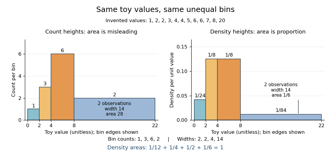

Bin choice trades detail against stability. Broad bins merge distinctions: the toy bin hides the empty stretch between and . Narrow bins expose gaps but can make each individual observation dominate a bar. With one-unit bins starting at , the bins each contain two values and appear equally prominent; that apparent pattern depends on grouping the repeated integers together. Moving the bin origin also changes membership without changing the observations. For density estimation, this is a form of the bias-variance tradeoff: averaging over broad bins loses local detail, while narrow bins give more variable density estimates across repeated statistical samples. [ref]
https://www.stat.cmu.edu/~cshalizi/uADA/24/lectures/ch14.pdf. Cosma Rohilla Shalizi, Estimating Distributions and Densities, Section 14.1
A useful practice is to compare a few plausible widths and offsets, keeping common edges when comparing groups. Automatic bin selectors are starting points, rather than guarantees of a unique correct picture. [ref]https://numpy.org/doc/stable/reference/generated/numpy.histogram_bin_edges.html. NumPy documentation, histogram_bin_edges, Notes on bin selectors
A histogram retains only bin membership. Its density estimate spreads each bin's fraction uniformly across that bin, so our last bar assigns density throughout even though the only toy values there are and . It does not recover within-bin positions or observation order, and a visually convincing shape does not establish a population probability distribution. A box plot provides a complementary compact summary of quartiles; neither graphic replaces the original observations.
Quartiles are the quantiles at probability levels ; is a median. For a population we can use its quantile function, for . Finite-sample conventions differ. Our box plot uses linear interpolation between order statistics: for and , setThen . This is R's type-7 convention, described in the documentation authored by Ivan Frohne and Rob J Hyndman. It differs from the generalized-inverse sample quantile defined elsewhere in this wiki: for the twelve toy values, that rule selects ranks and gives , rather than . These are different stated conventions, not arithmetic disagreements. [ref]
https://stat.ethz.ch/R-manual/R-devel/library/stats/html/quantile.html. Frohne and Hyndman, R stats documentation, sample quantile types
A box plot compresses a statistical sample into a box spanning its lower and upper quartiles , a line at its median , and two whiskers. It makes location and central spread easy to compare across groups on a common value axis. The box represents the central half in terms of quantile levels; with ties or interpolated quartiles, it need not contain exactly half the observations. Whisker endpoints require a stated convention: they can be the observed extremes, or they can stop short of separately marked observations. [ref]
https://www.itl.nist.gov/div898/handbook/eda/section3/boxplot.htm. NIST/SEMATECH, Box Plot, definition and variants
Here is one explicitly toy dataset, reused under histogram: twelve invented, unitless values, with repeated values counted separately, already arranged as order statistics:For this box plot we choose the interpolated quartiles defined under quartile, using R's type-7 rule. This givesThe interquartile range is . Our whisker convention uses the fencesThe whiskers end at the smallest and largest observations in the closed interval : here and . Values strictly outside the fences receive separate outlier markers: here only . An observation exactly on a fence is retained within the whisker under this convention. The fences are thresholds, not observed whisker endpoints; the upper whisker is at , not . R's documented whisker rule likewise includes observations no more than box lengths away, although its box uses hinges, which can differ from our type-7 quartiles. [ref]
https://stat.ethz.ch/R-manual/R-devel/library/grDevices/html/boxplot.stats.html. R grDevices documentation, boxplot.stats, coef and hinges
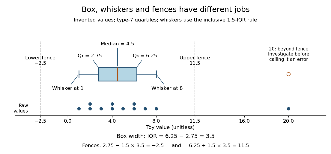

A separate outlier marker is a prompt to investigate, not a finding that the value is bad data and not an instruction to delete it. A distant observation can be a recording error, a legitimate unusual outcome, or evidence that the assumed statistical model misses some behavior. Check its provenance and context before deciding how to analyze it. No measurement-error claim is possible for our invented : we deliberately put it there to demonstrate the rule. [ref]
https://www.itl.nist.gov/div898/handbook/eda/section3/eda35h.htm. NIST/SEMATECH, Detection of Outliers, labeling and investigation
The beauty of a box plot is its compact comparison of ordered positions rather than every observation. That compression also loses information: many different statistical samples have the same quartiles and whiskers, so the box alone cannot reveal every cluster or gap that a histogram might show. For example, replacing the two invented values by and leaves the type-7 quartiles, whiskers and separate marker unchanged. Displaying the individual values alongside the box plot is especially helpful for such a small statistical sample. Always state both the quartile rule and the whisker rule; changing either can change which values are marked.
There are unlisted articles, also show them or only show them.