
On a star-shaped neighbourhood of , a smooth function satisfiesThe fundamental theorem of calculus along the segment proves the identity, and differentiation under the integral sign proves smoothness of the coefficients.
A formal pseudodifferential operator is a series in integer powers of , bounded above but possibly infinite towards negative powers. Its coefficients are smooth functions. Multiplication uses the formal pseudodifferential composition rule. Negative powers are formal inverses, not globally defined integration operators on all smooth functions. Every coefficient in a product is a finite sum, so multiplication is defined without analytic convergence.
For a commutative -algebra , a relative differential operator is a -linear endomorphism. Set , and define order at most by for every , where means multiplication by . Order zero is multiplication by an element of . The finite-order operators form the ring under composition. Specifying the base is essential: absolute operators on a complex polynomial ring include derivations of the coefficient field and need not be complex-linear.
Suitable curvature functions determine a regular Frenet curve up to a Euclidean rigid motion. In the plane one signed curvature suffices; in three dimensions positive curvature and torsion determine a unit-speed curve, as in the fundamental theorem of regular space curves. The result is local on the parameter interval and assumes the regularity needed by the frame equations.
The Dirichlet energy of a differentiable scalar function is one half the integral of its squared gradient. On a Euclidean domain it is ; the Dirichlet energy on a Riemannian manifold uses its metric and volume measure. Its stationary functions satisfy the Laplace equation with fixed boundary values.
Hodge theory connects de Rham cohomology with harmonic differential forms through the Hodge Laplacian on a compact Riemannian manifold. The Hodge decomposition theorem supplies a unique harmonic representative of each cohomology class. On a compact Kähler manifold, the decomposition additionally respects the complex bidegrees of differential forms.
On a graded nilpotent Lie group whose first layer generates its Lie algebra, a horizontal curve obeys for a control in the first layer. The displayed infimum is over horizontal curves with prescribed endpoints. The distance is left invariant and homogeneous under the graded dilations. On a free nilpotent Lie group it measures the least Euclidean length of a path realizing a prescribed truncated path signature.
Calibrated geometry constructs volume-minimizing submanifolds through closed differential forms with a tangent-plane bound. It gives an algebraic sufficient condition for solving the nonlinear minimal surface problem.
Imagine folding a sheet along its horizontal axis by the smooth map , . The inputs and have the same output. Along , horizontal motion still changes the output, but vertical motion produces no first-order change: . These inputs are critical points of a smooth map even though their differential is not the zero linear map. The missing direction in the target tangent space is what matters.
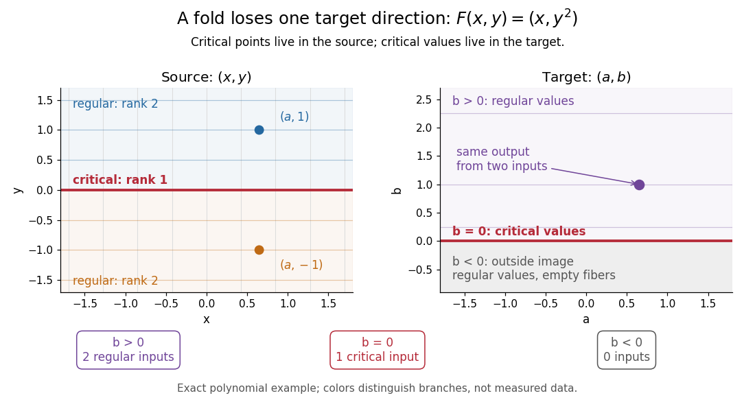
Precisely, let be a smooth map between smooth manifolds without boundary. An input is a critical point of a smooth map when its differentialis not surjective, equivalently when its rank of a linear map is less than . An input where it is surjective is a regular point; a map with no critical points of a smooth map is a submersion. The threshold is the target dimension, not . In manifold charts, compute the matrix rank of the Jacobian matrix; changes of charts preserve that matrix rank. [ref]
For the fold,Thus its set of critical points of a smooth map is the entire horizontal axis. Away from that axis, its differential can produce every infinitesimal target displacement. At the axis, it can produce only horizontal ones. This diagnoses where the two inverse branches in the picture merge.
For a scalar smooth function , the target dimension is one. A linear map to fails to be surjective exactly when it is zero, so here a critical point of a smooth map means . In Euclidean space this is precisely the familiar critical point condition : every first partial derivative vanishes. On a Riemannian manifold, it is equivalently for the chosen Riemannian metric; the Riemannian gradient depends on that metric, but whether it vanishes does not. See Loring W. Tu, An Introduction to Manifolds, Proposition 8.23 for the scalar coordinate criterion. The scalar smooth function has a critical point at zero without a local maximum or local minimum.
A source of lower dimension gives a different warning. For the smooth map , , the Jacobian matrix is the column , of matrix rank one at every input. Every input is a critical point of a smooth map, since the target dimension is two, even though this parametric curve has nonzero velocity everywhere and is an immersion. More generally, if , no differential can be surjective, so every input is critical. The terminology measures the ability to fill target directions, rather than whether the parametrized curve looks smooth.
This family includes the Laplace-Beltrami operator on functions, the Hodge Laplacian on differential forms, and the rough Laplacian associated with a connection on a vector bundle. Their domains and sign conventions must be specified when comparing them.
A smooth map between manifolds pulls a function back by composition and pulls a covariant tensor back by applying its differential to each vector argument. The pullback of a differential form is the alternating-tensor case and commutes with the exterior derivative.
The differential geometry of smooth surfaces studies their induced Riemannian metrics and intrinsic or extrinsic curvature. The first fundamental form measures lengths, while the second fundamental form and shape operator describe bending in an ambient Euclidean space. A regular parametric surface must have linearly independent tangent vectors : otherwise its parameters cannot provide a manifold chart with two independent directions.
For a sphere of radius , use colatitude and longitude :Thus a change has arc length : equally spaced longitudes draw closer together toward a pole. The coordinate degeneracy at the poles belongs to this parametrization, not to the smooth surface.
Both principal curvatures of the sphere have magnitude and the same sign, giving Gaussian curvature . A plane has , and a circular cylinder also has because one principal curvature vanishes. These three familiar shapes show why visible bending alone cannot measure intrinsic Gaussian curvature.
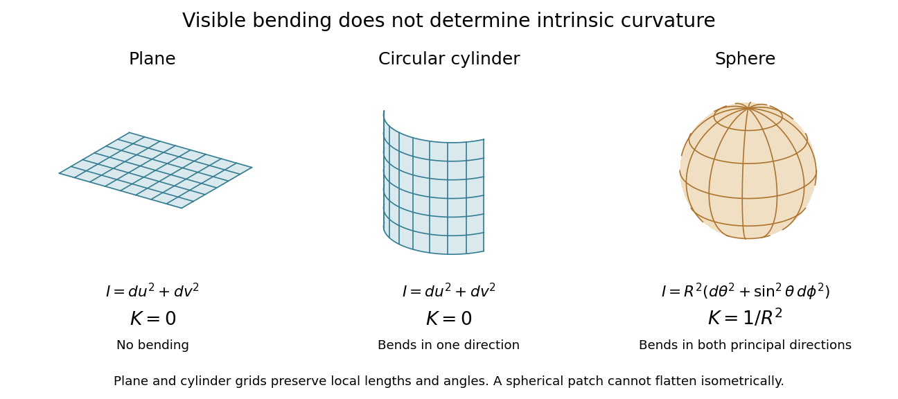
Visible bending and Gaussian curvature are different measurements
. Details. Let be a closed Riemannian manifold and a flat Hermitian vector bundle with unitary holonomy. On -valued differential forms of degree , let be the nonnegative Hodge Laplacian. For its positive eigenvalues, defineusing analytic continuation to ; the prime omits zero eigenvalues. The Ray-Singer analytic torsion isThis packages the form spectra into a regularized determinant, supplying an analytic counterpart of Reidemeister torsion.[ref]
For acyclic unitary coefficients on a closed manifold, this scalar is independent of the Riemannian metric. With nonzero cohomology, the scalar alone can depend on the metric; the full construction also tracks the norm of cohomology bases. For a circle of length with trivial coefficients, the positive eigenvalues are for in degrees zero and one. Their zeta regularization gives , illustrating that dependence.[ref]
R-torsion and the Laplacian on Riemannian manifolds by Daniel Ray and Isadore Singer. Section 2 for acyclic invariance; Section 3 for the nonacyclic construction
Turaev torsion refines the combinatorial side's sign and cellular-lift choices; comparing analytic and combinatorial constructions requires matching those conventions.
A differential 1-form is a smooth section of the cotangent bundle; it assigns a covector to every point of a smooth manifold. In planar coordinates, evaluates a tangent vector as .
Along a parametric curve , its line integral isReversing the direction reverses the integral. A force expressed as a one-form therefore accumulates work along a directed path. In Euclidean coordinates its components can be displayed as arrows, but identifying a one-form with a vector field uses an inner product; the covector field itself does not require a Riemannian metric.
For a smooth form of type , the complex orientation gives . Consequently its integral on a compact complex manifold is positive unless vanishes identically. Applying Stokes theorem to proves that a holomorphic differential form of degree on a compact complex -manifold is closed, without requiring a Kähler metric.
The comass is the operator norm of a differential form restricted to simple unit tangent multivectors. Reversing orientation gives the equivalent two-sided bound. It differs from the Euclidean norm of all the form's components. The calibration bound uses comass because tangent planes are represented by simple multivectors.
A compactly supported top-degree differential form on an oriented smooth manifold is integrated using orientation-preserving coordinates and a partition of unity. The coordinate change of variables formula makes the result independent of the choices. More generally, a form is integrated over a lower-dimensional oriented submanifold by its pullback. The Generalized Stokes theorem states with the induced boundary orientation. Integrating a closed differential form over a closed cycle depends only on its homology class, since its integral over a boundary vanishes.
A jump condition relates the one-sided limits of a solution or its derivatives across a discontinuity or singular forcing. Integrating a differential equation across a shrinking interval containing a Dirac delta source determines the permitted jump. A jump condition for an impulse and Rankine-Hugoniot condition are specific instances with different governing equations.
For the first-order ordinary differential equation defined on an open subset of the plane, an isocline of slope is the level setHere is a constant. At every point of this isocline, the direction field prescribes a tangent vector proportional to for a solution of a differential equation. It does not generally prescribe the tangent line of the isocline itself. The level set can have several components or fail to be a smooth curve, and points outside are excluded.
For example, take on the whole plane. Its isoclines are the parallel straight linesEach line has slope , while the direction field along it has slope . Thus the isocline carries horizontal segments even though the line itself rises. A function graph of a solution of a differential equation follows the segments, rather than following this line. Only the isocline with , namely , is also a solution of a differential equation.[ref]
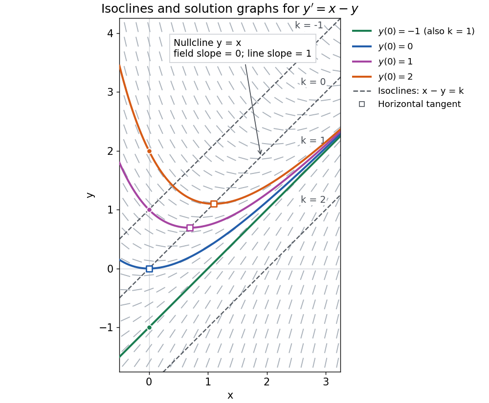


The first-order linear differential equation has the exact familyThe initial condition selects and hence a unique solution of a differential equation for every real . The picture shows . For the solution of a differential equation stays on the isocline; for other it moves through different isoclines. These formulas check the pictured trajectories by direct differentiation, independently of how the direction field was sampled.
The zero-slope isocline is called a nullcline. Below the nullcline in this example, ; above it, . For , the solution of a differential equation meets it at , where and , a strict local minimum. The nullcline is therefore a useful guide to turning points, although it is not itself a solution of a differential equation. In the equivalent planar autonomous differential equation , , it is the nullcline for the second component; there is no equilibrium point, because the first component never vanishes.
This makes isoclines useful even when no explicit solution of a differential equation is available: organize a direction field by common slopes, read where function graphs rise or fall, and identify possible turning points on nullclines.
There are unlisted articles, also show them or only show them.