Stars and bars counts tuples of nonnegative integers with a prescribed sum. For integers and , its statement isSuch a tuple is a weak composition of an integer. Think of labelled bins: counts identical objects in the first bin, in the second, and so on. Bin names distinguish positions even when counts agree. Stars and bars counts these count tuples; assigning individually distinct objects requires additional information. [ref]
https://math.mit.edu/~fgotti/docs/Courses/C.%20Combinatorial%20Analysis/6.%20Compositions/Compositions.pdf. Felix Gotti, MIT 18.211, Lecture 6: Compositions, Proposition 1 and Example 3
Computed example. With and , the number of weak compositions of an integer is . The string
••|•|•• encodes : two dots before the first bar, one between the bars, and two after the second. For a fixed first-bin count , the second-bin count can be any integer from to and the third is forced. Thus the direct count is .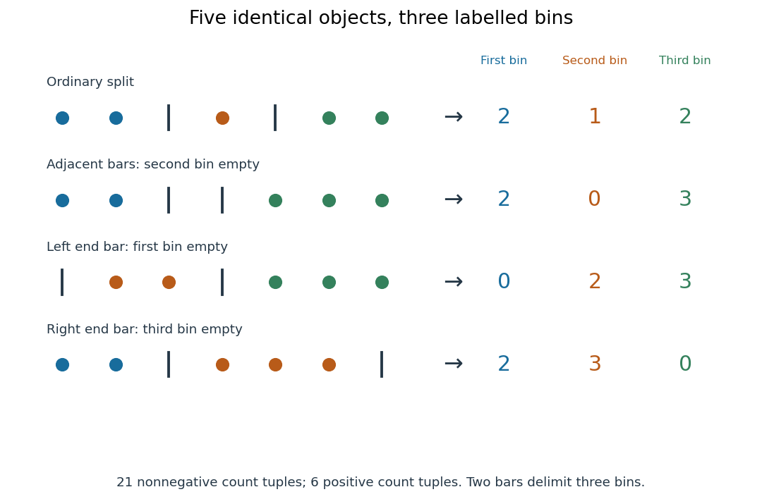
Stars and bars for five identical objects and three labelled bins: ordinary splits, adjacent bars, and bars at either end
. Details. Adjacent bars encode an empty middle bin:
••||••• gives . A bar at the left end encodes an empty first bin, as in |••|••• for ; a bar at the right end encodes an empty third bin, as in ••|•••| for . These are valid weak compositions of an integer. For every count is zero, and for the unique tuple is , consistent with .Proof outline. Replace each count by that many dots and separate successive groups with bars. Reading the group sizes reverses this construction, so it is a bijection between weak compositions of an integer and strings of dots and bars. Choose the bar positions among positions; the binomial coefficient counts the choices. The beauty is that empty bins need no separate cases: end bars and adjacent bars encode them automatically.
If every bin must be nonempty, the tuples are compositions of an integer, and their count is for ; for there are none. Subtract one from every count, setting . This is a bijection to weak compositions of an integer of , so stars and bars gives . For five objects and three bins, this is , with the six positive tuplesFor instance, shifts to , whose sum is . Sorting the six positive tuples collapses them to just two integer partitions, and . Thus named bins and unordered summands answer different questions.
Stars and bars is useful for allocating identical resources or enumerating integer solutions without listing them individually. Prescribed lower bounds can be subtracted just like the nonempty-bin requirement. Upper bounds require removing forbidden tuples; the existing bounded weak compositions article applies the inclusion-exclusion principle to those violations.
Double counting establishes an identity by computing the cardinality of the same finite set in two ways. The useful step is to identify exactly what the members of that collection are; an algebraic equality then records two legitimate ways to organize them.
Take the ordered pairs where is a -element subset of an -element set and is marked. Choosing first gives pairs. Choosing first leaves members to choose from the other , giving . HenceFor five people and two-person teams, both counts give : ten teams with two choices of a marked member, or five choices of that member with four choices of a teammate. The identity is explained by the bijection between these descriptions, rather than merely verified through factorials.
A tree is a nonempty connected graph containing no graph cycle. Think of seven locations joined so that everyone can reach everyone else, but no connection supplies an alternative route. For a finite simple graph with vertices, three descriptions are equivalent: being a tree; having exactly one simple graph path between every pair of distinct vertices; and being a connected graph with exactly edges. Here a simple graph path repeats no vertex. Connectedness in the last description is essential. [ref]
https://www.maths.tcd.ie/~dwilkins/Courses/MA2C03/MA2C03Courseware_2014to15/MA2C03_S4_Yr1415.pdf. Trinity College Dublin, graph theory notes, Theorems 4.24–4.26 and Corollary 4.27
For a concrete tree, label the vertices and take the edgeswhere abbreviates the unordered pair . There are seven vertices and six edges. The unique graph path from to is , using five edges. The degree sequence in label order is : its sum is , as the degree-sum formula predicts. Each of is a leaf of a graph, having vertex degree one.
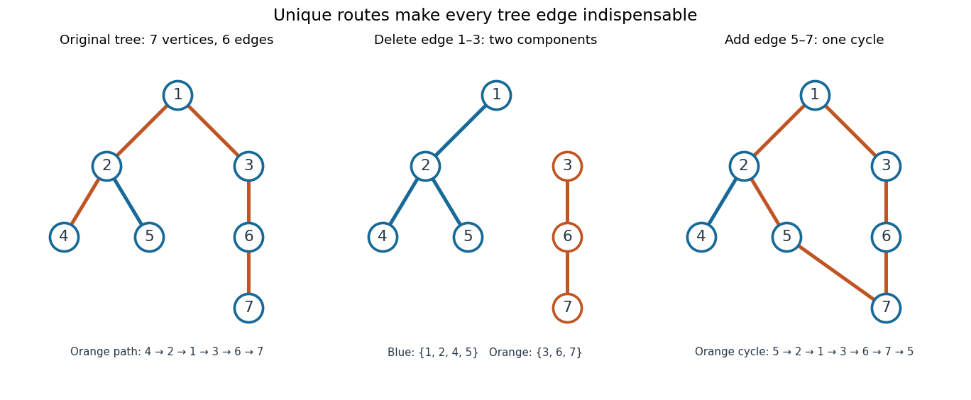
A seven-vertex tree: one graph path, two connected components of a graph after deletion, and one graph cycle after insertion
. Details. Deleting edge leaves precisely two connected components of a graph, on and . Every edge of a tree is a bridge in a graph. Instead add edge to the original tree: it closes the unique existing graph path into exactly one graph cycle. Thus a tree provides economical connections with no redundancy: a single failed link separates locations. Every finite tree with at least two vertices has at least two instances of a leaf of a graph; the endpoints of a longest graph path supply them. [ref]
https://www.mathstat.dal.ca/~janssen/2113/notes/class14/. Dalhousie University, Trees: leaves and indispensable edges
The number alone proves nothing about connectedness: a cycle graph on together with an isolated vertex has seven vertices and six edges, yet is disconnected. Briefly, two different simple graph paths between the same vertices would contain a graph cycle. Repeatedly removing a leaf of a graph and its incident edge proves the tree count by mathematical induction, starting with one vertex and no edges.
The indegree of a vertex is the number of directed edges entering it, counting repeated directed edges separately if permitted. In the toy directed acyclic graph, the initial indegrees of are . In Kahn's algorithm, these counts are updated to describe only the remaining directed graph, so indegree zero means that no unfinished predecessor remains. [ref]
https://raw.githubusercontent.com/kevin-wayne/algs4/master/src/main/java/edu/princeton/cs/algs4/Digraph.java. Sedgewick and Wayne, Digraph: definition of indegree
For finite sets, the number of ordered choices of one element from each is the product of the individual numbers of choices. More generally, if stage has exactly possible choices after every permitted history of earlier stages, the total number of full choice sequences is , by mathematical induction on the stages. This counts functions between sets of sizes , and counts the injective functions by the falling factorial when .
With five people, choose a captain in five ways and a different deputy in four ways: ordered assignments. The second choice depends on the first because the captain is excluded, but its number of permitted options is always four. The rule of product therefore applies without any assumption about independent events. To count two-person teams instead, each subset has two possible role assignments, so division by gives ten teams. This division works because every team was counted equally often.
A matroid is an independence system in which a smaller admissible selection can always grow using an element of a larger admissible selection. This exchange rule abstracts linear independence of vectors and the selection of edges forming a forest. It forces all matroid bases to have the same cardinality and makes the matroid greedy algorithm correct for maximizing their total weight. The useful surprise is that local choices become globally optimal because of a structural rule about admissible subsets, rather than a special numerical coincidence.
The weighted three-vector matroid below lets us inspect every subset and every possible size comparison. Its three vectors give three two-element matroid bases, yet their total weights differ. The graphic matroid of a graph triangle has exactly the same admissible labels. A pregeometry is a finitary closure-theoretic extension to possibly infinite sets.
A combinatorial structure is a discrete mathematical object specified by underlying elements and rules organizing them. A graph equips a set of vertices with edges; a permutation orders labels; a set partition groups them into nonempty subsets. Counting requires an explicit equality convention. Two labelled combinatorial structures may differ only by their labels, whereas an unlabelled combinatorial structure identifies objects related by an appropriate isomorphism. Thus there are three labelled two-element subsets of a three-element set, but only one abstract two-element set up to bijection.
Enumerative combinatorics counts families of finite combinatorial structures, usually as a function of size. Selecting labels from gives a binomial coefficient; arranging all labels gives a factorial; grouping labels gives a set partition. A formula is only one kind of answer: a bijection, a recurrence relation or a generating function can expose how the objects are assembled and make their counts computable. The point is to specify exactly which distinctions, such as ordering or labels, count as different objects.[ref]
In a two-level ground system, balancing collisional upward excitation against radiative and collisional downward loss gives . Excited lines fed in different proportions by these levels have a density-sensitive ratio. At low density the population ratio is proportional to density; at high density it saturates at . A reliable calibration uses a full multilevel model when upper-state branching and cascades matter.
Collision rate coefficient for an atomic transition by  Codex 0 Created 2026-10-13 Updated 2026-10-24
For a normalized electron speed distribution , the atomic transition rate coefficient is . Its dimensions are volume per time, so the rate per target atom is . Maxwellian detailed balance gives for .
College Physics by Paul Peter Urone and others 27.1 The Wave Aspect of Light: Interference by Codex 0 2026-10-13
Codex 0 2026-10-13Cited passages: section 27.1, wavelength in a medium: unchanged frequency and wavelength divided by refractive index.
A small organic helper involved in an enzyme's catalysis. It can be transformed in one chemical reaction and regenerated in another.
Time in physics orders physical events and measures durations between them. A clock realizes a time coordinate by counting a reproducible process, such as the oscillations of a simple pendulum. Describing a falling object's motion then means assigning a position to successive clock readings, making its velocity and acceleration measurable.
In Newtonian mechanics, a single common time parameter can be used throughout an experiment. In special relativity, the proper time accumulated by a particular clock depends on its world line, and assigning times to separated events requires a specified reference frame and clock synchronization. Two distant clocks therefore involve more physical structure than simply reading one local dial. The choice of a time origin is conventional; predictions concern durations and relations among measured events.
A mechanical constraint restricts the configurations or velocities a mechanical system can attain. A bead threaded on a rigid circular wire cannot move freely in three dimensions: the wire restricts its position to a circle, leaving one configuration degree of freedom. The supporting wire supplies a normal reaction that enforces this restriction.
A holonomic constraint can be expressed as an equation among configuration coordinates and possibly time, such as for a bead on a fixed circle. A nonholonomic constraint restricts allowed velocities without generally reducing to such a position equation; rolling without slipping can produce this situation. Using coordinates adapted to a mechanical constraint can remove unknown reaction forces from the equations of motion, while retaining the physical restriction they impose.
A torsion balance measures a weak torque by suspending a body from a thin fiber and reading its twist angle. The fiber supports the body's gravitational weight while permitting rotation about the suspension axis. In the range of linear elasticity, a twist in radians, measured from the untwisted reference orientation, produces a restoring torqueThe torsion constant sets the sensitivity. At static equilibrium with an applied torque and no other axial torque, . A perpendicular force at lever arm therefore gives . The torsion balance measures a turning effect: a force whose line of action passes through the suspension axis gives no axial torque. The Cavendish torsion balance is the gravitational application; Coulomb's law supplies an electrical one. [ref]
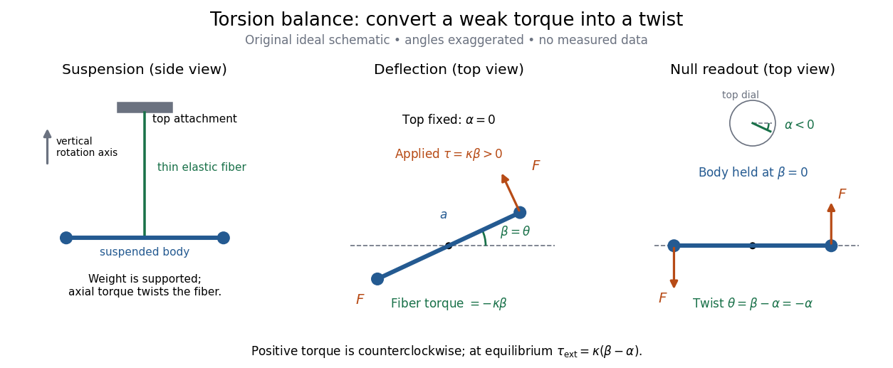


The original schematic separates two ways of reading the same torque. In deflection operation the top attachment stays fixed and the body rotates. In null operation the experimenter rotates the top attachment by while returning the body's laboratory angle to its original value. If the initially untwisted configuration has , the fiber twist is , not alone. ThusFor a positive applied torque, holding requires . Keeping the body at the same angle keeps the lever arm and source geometry fixed, making comparison of different applied forces easier. Either readout still requires a calibrated torsion constant and a stable reference orientation.
An illustrative calculation shows the amplification: with , , and , the applied torque is and the equilibrium twist is . These are stipulated values, not measured data. Reducing the torsion constant tenfold increases this twist tenfold, provided the fiber remains in its calibrated linear elasticity range. The cost is a slower response, explained by the oscillation period in torsion constant.
A concrete laboratory experiment is PASCO's Coulomb balance: level its counterbalanced rod, discharge both conducting spheres, and set the unloaded zero. Charge the spheres at maximum separation; switch off the charging supply. Move the second sphere to a known center separation , then turn the suspension dial until the rod returns to its index mark. Record the dial change and , recharge, and repeat at several separations. The manual recommends a draft-free room, clean insulating supports, and recharging before each reading: leakage, especially in humid conditions, otherwise changes the electric charges during the sequence. At close separations the conducting spheres redistribute charge, so the point charge approximation needs correction. [ref]
https://cdn.pasco.com/product_document/Coulombs-Law-Apparatus-Manual-ES-9070.pdf. Bruce Lee, PASCO ES-9070 manual, pp. 4–8: setup, force-versus-distance procedure, and corrections
For constant electric charges and a fixed perpendicular lever arm, the Coulomb's law prediction is . Plotting the logarithm of twist magnitude against the logarithm of separation gives , so the predicted slope is . Absolute force measurement additionally needs the torsion constant; comparing ratios can eliminate it if it remains stable. Repeating a reference separation between other settings distinguishes a separation effect from a changing signal. A declining reading at the reference separation would invalidate the assumption of unchanged electric charges, even if a distance plot looks smooth.
The historical electrical example is Coulomb's first memoir of 1785. His apparatus enclosed a suspended needle with a small ball and a second ball; an adjustable head twisted the suspension. After charging the balls by contact, he reported angular separations , , and with head settings , , and . The total twists were approximately , , and : fourfold restoring torque accompanied approximately halved separation. These are his reported observations, not data from our diagrams. [ref]
https://cnum.cnam.fr/pgi/redir.php?ident=8CA121-1&onglet=c. Coulomb, Premier mémoire (1785), reprinted in Mémoires de Coulomb, pp. 104–109, CNAM digitization
A precise reconstruction must use center distances and the changing lever arm, rather than identify angular separation exactly with distance; Alberto A. Martínez's replication explicitly analyzes that geometry. [ref]https://martinezwritings.com/m/Coulomb_files/CoulombExperiment-1.pdf. Martínez, Replication of Coulomb's Torsion Balance Experiment (2006), pp. 522–525
Sensitivity also exposes changes of the apparatus itself. Fleischer and colleagues' cryogenic torsion balance used a temperature-controlled enclosure to reduce vacuum-vessel top-plate temperature fluctuations to approximately , limiting changes in suspension geometry from thermal expansion. They used a mild bake-out near to speed initial fiber relaxation and reduce slow zero motion. Their optical readout compared the pendulum mirror with an internal reference mirror to reject shared optical motion. Room-temperature thermal radiation entering through the optical opening heated the pendulum; a cold filter reduced that load. The authors could not directly measure the pendulum's temperature without disturbing it, and explicitly distinguished the cold shield's temperature from the body's. Cooling therefore requires checking the actual noise and thermal environment, rather than assuming that the fiber and body share the shield's temperature. [ref]
A useful control strategy is to record unloaded readings and temperature before and after each signal sequence, recalibrate the torsion constant under the same conditions, and compare forward and reverse settings. The algebra of torsion balance zero drift shows precisely which offsets such comparisons can cancel. A fine angular scale alone does not establish a small measurement error.
The relational shape space of a particle configuration is obtained by removing collective translations and rotations; here scale is retained. For generic collision-free, noncollinear configurations of labelled particles in three dimensions, the resulting configuration dimension is . Collinear configurations have nontrivial rotational stabilizers and require singular strata. Removing position and orientation does not automatically remove conserved angular momentum or its centrifugal effect; a dynamically faithful reduction must retain the appropriate momentum-level data.
The configuration space of a mechanical system is the space of its allowed positions or generalized coordinates. Its tangent bundle describes configurations and velocities, and its cotangent bundle describes configurations and conjugate momenta. For smooth holonomic constraints it is a manifold on which geometric Lagrangian and Hamiltonian descriptions can be built. Singular constraints or symmetry quotients can require strata rather than one global smooth manifold.
There are unlisted articles, also show them or only show them.