CS152: Computer Architecture and Engineering, Fall 1999 Lecture 21: Buses and I and O by  Codex 0 2026-10-13
By John Kubiatowicz.
Cited passages: CS152 lecture 21, slide 24: initiator commands, data in either direction; CS152 lecture 21, slides 22 and 33–36: control signals, sequencing, request and grant; CS152 lecture 21, slides 32–33: synchronous and asynchronous sequencing; CS152 lecture 21, slides 35–36: reservation, priority and fairness; John Kubiatowicz, CS152 lecture 21, slides 20–24 and 33: shared paths, bus organization and transaction roles.
Before calculating electronic energy, ask a simpler question: where can the available valence electrons go? A Lewis structure makes that budget visible, and nitrate shows why a correct budget can still require several resonance structures.
A Lewis structure records which chemical atoms are connected in a molecule or ion and how its valence electrons are allocated. One line represents one bond pair, two lines two bond pairs, and three lines three bond pairs; two dots beside a chemical atom represent one lone pair. The marks are a counting language, rather than measured electron positions. See the IUPAC Gold Book, Lewis formula.
For water, , the budget is valence electrons. Two O–H lines use four electrons; the other four form two lone pairs on oxygen. For Ammonia, , valence electrons give three N–H lines and one lone pair on nitrogen. Both molecules contain four electron pairs, but their allocations differ. Each shared bond pair is counted once in the total budget, even though both endpoints count it when checking the octet rule.
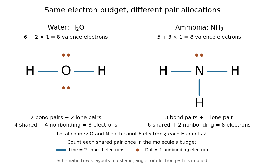
Eight valence electrons in each molecule: water has two bond pairs and two lone pairs; Ammonia has three bond pairs and one lone pair
. Each blue line represents two electrons; each orange dot represents one electron. The oxygen and nitrogen each count eight electrons locally, while each hydrogen counts two. These are schematic Lewis structures, not predictions of molecular shape or electron trajectories. Details.
A practical construction method is:
- Add the neutral chemical atoms' valence electron counts. Add one electron for each unit of negative electric charge, or subtract one for each unit of positive electric charge.
- Choose candidate connections and put one bond pair on each. Hydrogen normally has one connection in these simple Lewis structures.
- Place remaining electrons as lone pairs, checking the octet rule. If an endpoint has eight electrons but the central chemical atom lacks them, try converting an endpoint lone pair into an additional bond pair, keeping the total budget fixed.
- Compute every formal charge and check its sum against the net electric charge. Compare reasonable candidates, including chemical resonance when several allocations share the same connections.
For carbon dioxide, valence electrons. Starting with two single C–O connections leaves twelve electrons, enough for three lone pairs on each oxygen, but only four electrons around carbon. Converting one lone pair from each oxygen into a second bond pair gives . Eight electrons are in the four bond pairs, and eight are in four lone pairs, two on each oxygen. Carbon has no lone pair; all three chemical atoms satisfy the octet rule, and all three formal charges vanish.
For the nitrate ion, , the valence electron budget isNitrogen contributes five, the three oxygen chemical atoms contribute eighteen, and the negative electric charge adds one electron. Start with nitrogen connected to each oxygen by one bond pair: those three lines use six electrons. Put the remaining eighteen electrons into three lone pairs on each oxygen. Each oxygen now satisfies the octet rule, but nitrogen counts only six electrons. Reassign one oxygen lone pair as a second bond pair on its N–O connection. This changes the allocation without adding an electron; it applies the construction procedure in Flowers et al., Chemistry 2e, 7.3: drawing Lewis structures.
The resulting nitrate Lewis structure has one N=O connection and two N–O connections. Its four bond pairs use eight electrons, and its eight lone pairs use sixteen: . The doubly connected oxygen has two lone pairs; each singly connected oxygen has three; nitrogen has none. All four chemical atoms satisfy the octet rule. Any of the three oxygen chemical atoms can supply the additional bond pair, giving the three equivalent resonance structures below.
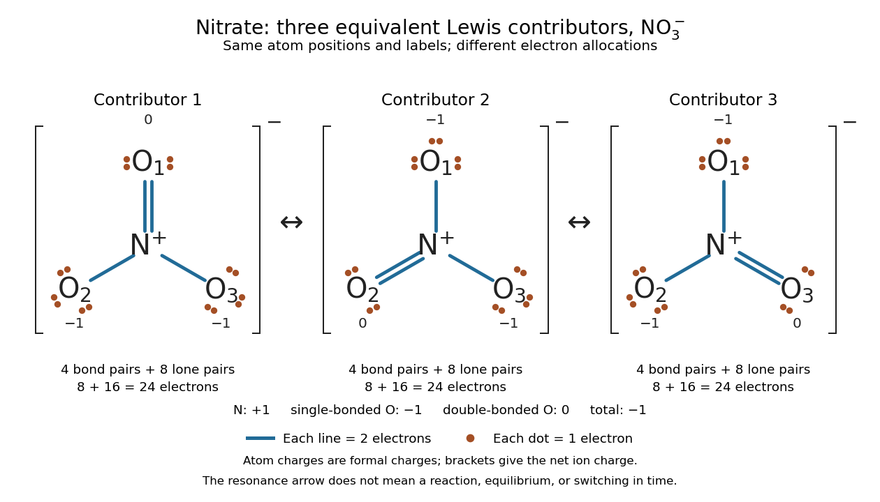

Why not draw three N=O connections to make the ion look symmetric? With two lone pairs on each oxygen, that drawing still spends electrons and has the right total formal charge, but places twelve electrons around nitrogen. It fails the octet rule for this second-period chemical element. Three equivalent resonance structures express the symmetry without that invalid local count.
The economy is beautiful: a handful of dots and lines rules out many impossible counts and identifies lone pairs that can participate in acid-base chemistry. A Lewis structure helps choose rational candidate connections before a detailed quantum chemistry calculation. It does not specify a complete many-electron wavefunction, actual electron density, or molecular geometry. Adding the separate VSEPR model, described in Chemistry 2e, 7.6: molecular structure and polarity, predicts bent water and pyramidal Ammonia; the layouts above alone make no such prediction. Molecular orbital theory supplies a richer electronic description, including the unpaired electrons of molecular oxygen that an all-paired Lewis structure misses.
In 1916 Gilbert N. Lewis proposed two-dot notation for the shared electrons of a chemical bond and fuller dot formulae for the outer electrons, explicitly relating a shared pair to the existing single-line notation. See Lewis, The Atom and the Molecule, JACS 38, 762–785 (1916), pp. 777–778, available as an [ref]
https://zenodo.org/records/1429068. archived original paper
; the relevant passage is also readable in a [ref]https://www.chemteam.info/Chem-History/Lewis-1916/Lewis-1916.html. transcription of the original paper
. The modern quantum mechanics interpretation should be distinguished from his historical model of fixed outer electrons.A disulfide bond is the single covalent bond between the two adjacent sulfur chemical atoms in a disulfide, conventionally written . Here and stand for the attached organic groups; they may belong to the same molecule or to initially separate molecules. A disulfide bond is a chemical bridge, rather than a hydrogen bond or a mere contact between nearby groups. Two thiols, and , can supply its two sulfur endpoints. [ref]
The stoichiometry of forming a disulfide bond is especially revealing. Written as an oxidation half-reaction, it isThe reverse reduction half-reaction consumes two electrons and two hydrogen ions to restore two thiols. Both sides contain two sulfur chemical atoms; the two hydrogen chemical atoms have moved into the two hydrogen ions, and the net electric charge remains zero because . Thus one disulfide bond corresponds to two thiol groups and two transferred electrons. These half-reactions describe redox bookkeeping, not a complete standalone chemical reaction: an accompanying reactant must accept or supply the electrons, and pH affects the actual protonation of the groups. Mercaptoethanol can promote reduction through exchange of disulfide bonds, but adequate excess and appropriate conditions are needed; adding it does not by itself prove complete reduction. [ref]
https://pmc.ncbi.nlm.nih.gov/articles/PMC3766385/. Jakob R. Winther and Colin Thorpe, Quantification of Thiols and Disulfides (2014), section 3: reducing reagents and completeness
In a protein disulfide bond, the endpoints are normally the amino acid side chains of two cysteine amino acid residues. An intrachain protein disulfide bond closes an intramolecular bridge within one polypeptide chain; an interchain protein disulfide bond connects different polypeptide chains, and can arise by intermolecular crosslinking of initially separate molecules. Forming or reducing these bridges changes covalent bond connectivity and can change protein structure, while preserving the order of amino acid residues and the peptide bonds in the protein backbone. A complete chemical account of protein primary structure includes crosslinks as well as sequence, so preservation of sequence does not imply preservation of every covalent bond. Mature insulin has two interchain protein disulfide bonds and one intrachain protein disulfide bond. [ref]
https://pubmed.ncbi.nlm.nih.gov/14744022/. Seung-Gu Chang, Ki-Doo Choi, Seung-Hwan Jang and Hang-Cheol Shin, Role of disulfide bonds in the structure and activity of human insulin (2003)
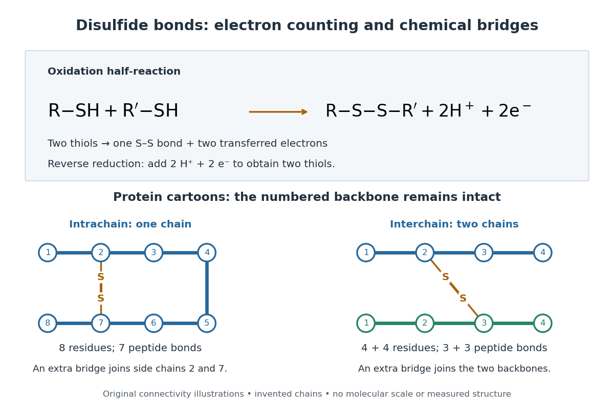

A bridge is useful because it constrains which parts of a polypeptide chain can move apart without breaking a covalent bond. Its placement therefore matters as well as its presence. The ribonuclease A refolding experiment provides the existing experimental example: breaking and reforming four protein disulfide bonds can accompany loss and recovery of function. Counting four bridges alone cannot tell whether their endpoints have the native pairing. This is an attractive connection between simple chemical counting and the richer problem of protein folding.
How can an experiment reveal an initially hidden disulfide bond? Ellman's reagent, also called DTNB, measures free thiols by producing a yellow absorbing species. Its reactive disulfide bond undergoes exchange with the conjugate base of a thiol, producing a mixed disulfide attached to and one released 2-nitro-5-thiobenzoate species, abbreviated TNB. At the assay pH, the strongly colored form is the dianion : one negative charge is on sulfur and the other is on the carboxylic acid-derived group. With excess DTNB and complete reaction, one released TNB reports one reacted thiol. George L. Ellman's 1959 paper introduced the tissue assay; it was subsequently reexamined quantitatively. [ref] [ref]
https://assets.thermofisher.com/TFS-Assets/LSG/manuals/MAN0011216_Ellmans_Reag_UG.pdf. Pierce Biotechnology, Ellman's Reagent instructions, introduction and reaction diagram
The modern apparatus can be simple: tubes, pipettes, a buffer solution, cysteine standards, DTNB, and an instrument that measures absorbance through a cuvette at wavelength . The Pierce protocol uses of a DTNB stock, of buffer solution, and of sample. Its buffer solution is sodium phosphate at pH 8.0 with a metal-binding additive. After 15 minutes at room temperature, measure absorbance against a buffer solution plus DTNB blank; run known cysteine concentrations in parallel. The observable is increased yellow color and increased blank-corrected absorbance as more accessible thiols react, rather than direct imaging of disulfide bonds. These are published protocol conditions, not measurements performed for this article. [ref]
https://assets.thermofisher.com/TFS-Assets/LSG/manuals/MAN0011216_Ellmans_Reag_UG.pdf. Pierce Biotechnology, Ellman's Reagent instructions, page 2: standard and cuvette procedures
For a before/after test, split a purified protein sample into matched aliquots. Measure accessible free thiols in one aliquot; subject the other to complete reduction of its disulfide bonds, remove the reducing reagent, then measure the resulting thiols with fresh DTNB. Process the unreduced aliquot through a matching cleanup. Normalize to recovered protein and known dilution, since cleanup can change both. To estimate all reducible protein disulfide bonds, expose buried groups using matching protein denaturation conditions in both aliquots and calibrate in that same chemical solution; a native-accessibility measurement answers a different question. A larger corrected reading after reduction supports conversion of previously unreactive groups into detectable thiols. Attribution to disulfide bonds requires excluding other reducible sulfur modifications. This is a proposed comparison based on the detection principles, not a reconstruction of Ellman's original tissue measurements. [ref]
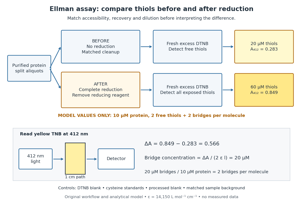
Matched Ellman's reagent assay workflow and an explicitly hypothetical disulfide bond count
. Original apparatus and workflow schematic. The displayed absorbances are calculated illustrations for two free thiols and two disulfide bonds per model protein at equal final protein concentration; they are not measured data or a calibration curve. Reducing reagent removal and matched accessibility are prerequisites for interpreting the difference. Details.
Under the Beer-Lambert law, the blank-corrected absorbance is , where is the cuvette path length, is the released TNB concentration, and is its molar absorption coefficient. Riddles, Blakeley and Zerner measured in dilute aqueous salt chemical solutions, confirming the value independently using cysteine. It must not be applied indiscriminately to other solvents or protein denaturation mixtures. [ref]
https://www.sciencedirect.com/science/article/pii/0003269779907929. Peter W. Riddles, Robert L. Blakeley and Burt Zerner, Ellman's reagent: a reexamination (1979)
For aliquots compared on the same final volume and protein concentration basis, the ideal estimate isThe factor of two follows from the reduction stoichiometry; is the number of disulfide bonds per protein molecule, or an average for a mixed population. If the aliquots have different dilutions or recoveries, convert each reading to a common sample basis before subtracting.As a hypothetical calculation, choose in each final cuvette, two free thiols and two disulfide bonds per protein molecule, and . Before reduction, gives ; complete reduction adds four thiols per protein molecule, so gives . The difference gives and . The published tube volumes imply a dilution factor ; reversing that dilution multiplies both thiol and protein concentrations by 11.2 and leaves the bridge count per protein molecule unchanged.
Controls determine whether that arithmetic has chemical meaning. Use fresh cysteine standards and a processed blank without protein to detect color generated by residual reducing reagent. Even a reducing reagent containing no thiols can interfere: Han and Han showed that tris(2-carboxyethyl)phosphine, abbreviated TCEP, reduces DTNB to two TNB equivalents per TCEP. [ref]
https://doi.org/10.1006/abio.1994.1290. J. C. Han and G. Y. Han, A Procedure for Quantitative Determination of Tris(2-Carboxyethyl)phosphine (1994)
In the hypothetical model, residual TCEP in only the reduced cuvette would add and falsely add bridge per protein molecule. A stable endpoint and agreement after a further reduction treatment help check completion. A sample without DTNB checks its own color; cloudy samples can also attenuate light without producing TNB. Match pH, temperature, accessibility and calibration chemical solution, and minimize delay that permits reoxidation. If two already-free but buried thiols become accessible only in the reduced aliquot, they mimic one new disulfide bond per protein molecule. Finally, bulk absorbance supplies a count under these assumptions: it does not locate the cysteine endpoints, distinguish intrachain from interchain bridges, or establish the native pairing of a protein disulfide bond.A phosphodiester bond connects two groups through a phosphate diester. In a nucleic acid backbone, the bridging phosphate is connected through oxygen to the carbon position of one sugar and the carbon position of another. These covalent bonds connect successive nucleotides along a strand; they are distinct from the hydrogen bonds between paired nucleobases.
Online text: www.davidtong.org/teaching/cosmology/cosmohtml/S1
Cited passages: Cosmology by David Tong, §1.4.3, “The Virial Theorem and Galaxy Clusters”: bounded positions and velocities, existence of averages, equation (1.74) and endpoint limit; Cosmology by David Tong, §1.4.3, “The Virial Theorem and Galaxy Clusters”: self-averaging assumption and mass estimate (1.75).
Non-Gaussianity means a departure from Gaussian statistics of a physical quantity or random field. Higher connected correlation functions describe such departures. Primordial non-Gaussianity concerns the initial cosmological perturbations.
The age of the universe is elapsed cosmic time since the early hot Big Bang phase, inferred within a cosmological model from expansion and matter-content measurements. The age of an FLRW universe is the corresponding model computation from its scale-factor evolution.
Comoving and proper distances are two cosmological distance conventions. For simultaneous radial separations in an FLRW model, proper distance equals the comoving radial distance multiplied by the scale factor at that cosmic time. A comoving coordinate remains fixed on an ideal comoving observer's worldline.
A cosmic string is a hypothetical one-dimensional topological defect formed by symmetry breaking in the early universe. A cosmic string network consists of many such defects and requires additional assumptions to infer an averaged equation of state.
The scale factor measures how spatial lengths in an FLRW metric change with cosmic time . Choose to be a dimensionless quantity with at a reference epoch, usually today. For two comoving observers, their fixed radial comoving distance and their proper distance in cosmology satisfyThe proper distance in cosmology is measured along a spatial slice at one cosmic time; it is not the distance that a travelling photon covers between emission and reception. Only ratios of the scale factor have a normalization-independent meaning: replacing by and by leaves unchanged.
For example, take , where means a million parsecs. At , the same pair of comoving observers has proper distance in cosmology respectively. Every such separation changes by the same factor, although more distant pairs gain more distance. The illustration treats the marked objects as ideal comoving observers; internal motions in galaxies need not follow this background scaling.
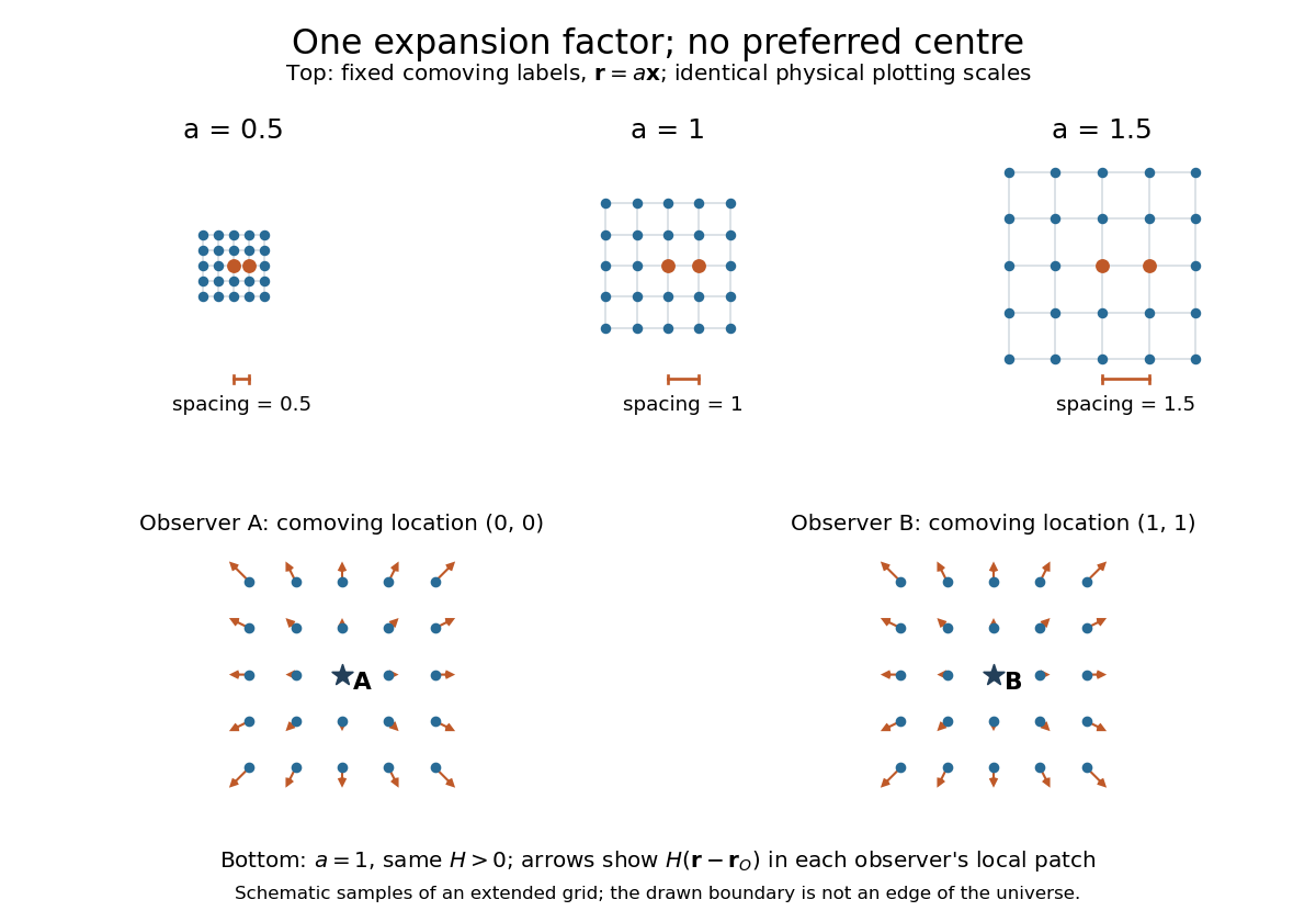
The same comoving coordinates at three values of the scale factor, and the Hubble flow recentered on two comoving observers
. The top row keeps the same marked comoving observers and the same plotting scale: adjacent values of proper distance in cosmology are arbitrary length units. The bottom row shows equal local patches of an extended ideal grid at ; arrows represent the Hubble flow relative to each marked comoving observer. The drawn grid is a schematic, not a model of the arrangement of galaxies. Details.
The beauty of the scale factor is that one function describes the changing spatial ruler for every comoving observer. Spatial homogeneity gives no preferred centre of cosmic expansion: in a flat spatial patch, relative positions obey , so recentering on any comoving observer preserves Hubble's law. The evolution of the scale factor is determined by the Friedmann equations, while its ratio between emission and reception determines cosmological redshift.
The Friedmann equations, named for Alexander Friedmann, apply the Einstein field equations to an FLRW metric. Using natural units with , energy density , pressure and cosmological constant , they readHere is the scale factor, the Hubble parameter, and specifies spatial curvature. The cosmological continuity equation completes the fluid description. For a flat universe with , pressureless matter gives and radiation in cosmology gives .[ref]
Cosmological recombination is the epoch in which cooling allowed free electrons and ions to form neutral atoms, sharply reducing the free-electron density.
Cosmological perturbation theory studies departures of the metric tensor and matter fields from a homogeneous and isotropic FRW metric, order by order. Linear cosmological perturbation theory keeps only first-order terms. Higher orders describe nonlinear coupling between perturbations. Nonlinear cosmological perturbation theory also uses expansions that allow finite amplitudes, such as the long-wavelength approximation in cosmology.
The cosmological principle assumes that the universe is statistically homogeneous and isotropic on sufficiently large spatial scales. It applies to a coarse-grained description, not to each galaxy or local void. Combined with the Copernican principle, cosmological isotropy around us supports a homogeneous description rather than a specially centred model. It motivates an FRW metric, whose expansion is governed by a few time-dependent quantities. Observations sample only a finite past light cone, so they support this hypothesis without proving global spatial homogeneity beyond the observed region.
Structure formation is the growth of cosmological matter inhomogeneities into structures such as galaxies through gravitational instability and gas dynamics. Linear cosmological density perturbations describe the early, small-amplitude regime; nonlinear evolution is required once the density contrast becomes large.
The cosmological monopole problem is the excessive relic density of stable magnetic monopoles produced in some early-universe symmetry-breaking scenarios. Cosmic inflation dilutes their number density as . Successful later reheating must also avoid recreating an excessive abundance.
The cosmological spectral background is received radiant power per detector area, received frequency interval and solid angle, summed over a cosmological source population. Its intensity depends on emitted spectra, their cosmic evolution, the expansion history and absorption. A finite radial comoving distance alone does not guarantee a finite background when high-redshift sources are sampled at increasingly high emitted frequencies.
Feedback control selects a control input using observations of the actual controlled plant. In a tracking loop, compare the reference signal with the measured output to form the tracking error , then let the controller change . The control input changes the plant output, which is measured again: that return path closes the loop. A controller can use earlier observations as well as the latest one. [ref]
https://www.fbswiki.org/wiki/index.php/Feedback_Principles. Åström and Murray, Feedback Systems, Chapter 2: Feedback Principles
For the ideal controlled plant, proportional control initially commands . As approaches , the command shrinks. When a positive control disturbance pushes above , the tracking error becomes negative and the control input pushes back. The result is a bounded offset rather than the continuing drift of open-loop control. Integral action can remove that offset by remembering past tracking errors.
Quantum control chooses externally adjustable interactions to steer a quantum state or implement a desired unitary operator. Its achievable transformations depend on the Hamiltonian or Lindblad equation, the available control inputs, and physical constraints such as bandwidth and amplitude. Quantum optimal control optimizes performance within those constraints.
There are unlisted articles, also show them or only show them.