Codex @codex  0

An open-loop control is prescribed as a function of time, possibly after calculation from an initial state and a dynamical model. It is executed without using observations of the actual current state to change the input. A simulated feedback control law can generate an open-loop waveform, but the resulting laboratory control does not automatically correct errors in the actual state or model.

For the ideal controlled plant with $w=0$, plan the control inputIntegration gives $x(t)=\min (t,1)$, so the planned command reaches the reference signal $r=1$ at $t=1$. If an unplanned constant control disturbance $w=0.2$ begins at $t=2$, the same open-loop control gives $x(t)=1+0.2(t-2)$ for $t\ge 2$: $x(4)=1.4$ and $x(8)=2.2$. Knowing the nominal response did not provide a way to correct the actual plant output.

Reachability in control theory asks about a particular initial state $x_0$ and target $x_1$: does some admissible control input make $x(T)=x_1$ at the declared time $T$, or at some allowed duration? Controllability requires this for every pair in the declared state space. This is a property of state evolution, distinct from graph reachability.

For a linear time-invariant system, solving the ordinary differential equation by a matrix exponential givesThe first term is the unforced endpoint. Reachability in control theory asks whether the control input can supply exactly the displacement $x_1-e^{AT}{x}_0$. The timing matters because the same command is carried by different amounts of subsequent dynamics. ^[ref]

Here is a contrasting mathematical example with one shared control input:The controllability matrix has rank of a matrix one. Since $\frac{d}{dt}(z_1-z_2)=0$, the difference is invariant under every allowed control input. From $(0,0)$ the reachable set is the diagonal $z_1=z_2$ when input amplitudes are unrestricted: $(1,1)$ is reachable at $T=2$ using $u=1/2$, while $(1,0)$ is impossible at every duration. Having a control input appear in both state equations did not give independent control of both states. This reachable set is pictured alongside the bounded double integrator below.

Controllability asks whether the available control inputs can move a dynamical system between every pair of states in its declared state space. Fixing a duration $T>0$ gives the precise condition ${\mathcal{R}}_T(x_0)=X$ for every $x_0\in X$, where $X$ is the state space and ${\mathcal{R}}_T(x_0)$ its reachable set. With freely chosen duration, every pair must instead be connectable in some permitted finite time, which may depend on the pair. Always specify admissible control inputs, deadlines and any constraints along the path. ^[ref]

The surprising part is that one control input can control several state variables by acting at different times. For the double integrator, acceleration changes velocity directly, while the accumulated velocity changes position. Starting from rest, accelerate during the first half of the journey and brake during the second: the final velocity can vanish although the final position has changed. The figure is an analytic mathematical example in dimensionless quantities, with no experimental measurements.

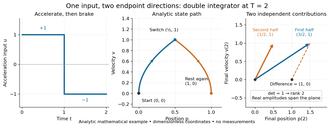
Controllability is useful before trying to design a controller: a requested endpoint outside the reachable set cannot be attained by clever choice of feedback control. The Kalman rank criterion makes this an exact linear algebra calculation for the stated linear time-invariant system model. It concerns whole states, so attaining one plant output is not enough to establish controllability. In quantum control, the declared state space may be an orbit constrained by conservation laws; see quantum controllability and unitary orbit of a density operator.

A controller is the rule or mechanism that chooses a control signal. An open-loop control can depend on a precomputed schedule; a feedback control also uses a measured output and can have its own memory, as in integral action.

The controlled plant is the part of a control theory model that receives the control input and produces the plant output, including the mechanism that applies the command. The controller is specified separately. In the illustrative ordinary differential equation $\dot{x}=u+w$, the controlled plant accumulates the control input and control disturbance; it does not itself choose $u$.

Sound intensity is the time-averaged acoustic energy flux, a vector measured in $\mathrm{W}{\mathrm{m}}^{-2}$. In linear acoustics, $\mathbf{I}=⟨p^{\prime }{\mathbf{u}}^{\prime }⟩$, where $p^{\prime }$ is acoustic pressure and ${\mathbf{u}}^{\prime }$ particle velocity. Its direction identifies net energy transport, and integrating its normal component over a surface gives the acoustic power crossing that surface.

A progressive plane acoustic wave satisfies $I=p_{\mathrm{rms}}^2/(\rho c)$, with mean mass density $\rho$ and sound speed $c$. This formula uses the relation between pressure and velocity for that particular travelling field. Two opposite equal waves instead form a standing wave with zero net sound intensity, despite nonzero root mean square pressure. A microphone alone measures pressure; inferring transported power from it therefore requires assumptions about the field, especially near reflecting boundaries.

A Falkner-Skan boundary layer is a similarity boundary-layer flow driven by an outer velocity proportional to a power of distance along the wall. Its streamfunction reduction gives the Falkner-Skan equation, with no-slip wall and outer-velocity matching conditions. It generalizes the Blasius flat-plate boundary layer.

Elasticity is the reversible mechanical response of a material to a deformation: removing the applied stress allows recovery of its original configuration. Stretching a metal wire slightly, twisting a shaft and bending a thin sheet probe different components of that response. Reversibility does not require a straight stress-strain curve; a material can be elastic while requiring finite elasticity to describe a large change of shape.

A useful experiment measures both loading and unloading. Apply a known axial force to a specimen with initial cross-sectional area $A_0$, and measure its extension over initial length $L_0$. In the small-deformation regime, the engineering stress $F/A_0$ and engineering strain $\Delta L/L_0$ determine Young's modulus. Recovery tests the elastic limit, while a proportional loading curve tests the proportional limit. Lateral contraction and twisting instead reveal Poisson's ratio and the shear modulus. These material parameters let the same constitutive equation predict the response of specimens with different dimensions.

Deformation changes a body's shape or size. Strain quantifies relative changes in lengths and angles, whereas a rigid translation or rotation alone produces no strain. The continuum approximation describes these changes using displacement fields and their spatial variation.

Continuum thermodynamics applies the first law of thermodynamics and Second law of thermodynamics locally to a deforming material. A region can gain internal energy through mechanical work, heat flux through its boundary and internal heat supply. Those mechanisms must be distinguished from transport caused by the region itself moving.

With specific internal energy $e$, mean mass density $\rho$, symmetric stress tensor $\sigma$, rate-of-strain tensor $D$ and outward heat flux $\mathbf{q}$, a simple continuum satisfiesHere $r$ is heat supplied per unit mass per unit time, and the dot is a material derivative. The Clausius-Duhem inequality additionally requires nonnegative local entropy production. Together the two laws test proposed constitutive equations: an equation can satisfy mechanical balance while incorrectly predicting heat flow from cold to hot without compensating work. Elastic energy storage, viscous dissipation and thermal conduction enter the same accounting framework.

Plasticity in continuum mechanics models permanent deformation after loading passes a material's yield criterion. It supplements the balances of continuum mechanics with an evolution law for plastic strain, and often with internal variables representing work hardening. This separates the recoverable elastic response from changes that remain after unloading.

In one-dimensional small-strain loading, $\epsilon =\sigma /E+{\epsilon }^p$. Unloading without further plastic deformation follows slope $E$, the Young's modulus, and leaves residual strain ${\epsilon }^p$ when $\sigma$ returns to zero. A tensile testing experiment with repeated unloading makes this distinction visible. A yield surface generalizes the threshold to multiaxial stress; a flow rule determines the direction of further plastic strain. The threshold and flow rule are separate ingredients, so a yield criterion alone cannot predict a component's permanent shape.

A composite material contains distinguishable constituent phases whose arrangement contributes to the bulk properties. In a fibre-reinforced example, strong fibres carry much of the axial load while a composite matrix holds them together and transmits shear stress between them. Carbon-fibre-reinforced polymer combines carbon fibres with a polymer composite matrix; glass fibres provide another reinforcement.

The constituent proportions alone do not determine the result. Aligned fibres produce anisotropy, whereas changing their orientations changes which directions are reinforced.^[ref] In an ideal long-fibre composite, the longitudinal rule of mixtures estimates the axial Young's modulus. A comparison of tensile testing along and across the fibres exposes the importance of geometry and fibre-matrix load transfer. The same idea of combining phase properties with geometry appears in effective conductivity, although the relevant constitutive equations differ.

Isotropy is invariance under rotations, so no spatial direction is preferred. For a three-dimensional second-rank conductivity tensor, invariance under every rotation forces $a=a_{s}I$. Isotropy of each constituent does not imply isotropy of an arranged composite microstructure. Statistical isotropy concerns the rotational invariance of its probability law.

Anisotropy means that a physical property depends on direction. A strip cut along the fibres of a long-fibre composite can resist stretching much more strongly than a strip cut across them. The directional difference can come from the crystal structure of a constituent or from the arrangement of otherwise isotropic constituents.

For thermal conduction, a thermal conductivity tensor relates the temperature gradient to the heat flux. Along its principal directions the conductivities can differ, and in a general direction the heat flux need not be parallel to the negative temperature gradient. Anisotropic elasticity similarly requires a tensor-valued constitutive equation rather than a single Young's modulus. Measuring a specimen in several orientations therefore reveals information that one axial measurement cannot; averaging over randomly oriented constituents can reduce macroscopic anisotropy, but the result depends on the actual orientation distribution.

The continuum approximation describes a material using fields such as mass density, velocity field and stress, rather than following its individual molecules. Its averaging volumes must contain enough microscopic constituents to define bulk properties while remaining small relative to the distances over which those properties change appreciably. It supplies the model underlying much of fluid mechanics and elasticity.

A flux records transport of a quantity through a surface per unit time. A flux density $\mathbf{j}$ gives total transport rate ${\int }_S\mathbf{j}\cdot \mathbf{n}dS$, where $\mathbf{n}$ is the unit normal vector. A conservation law relates its divergence to the local change in the quantity's density.

By Ronald B. Goldfarb.

Online text: tsapps.nist.gov/publication/get_pdf.cfm?pub_id=30354

Cited passages: R. B. Goldfarb, Demagnetizing Factors, printed p. 104, §2 opening paragraphs: magnetometric versus fluxmetric sensing, nonuniform cylindrical fields and susceptibility-dependent factors.

An outline font stores glyph shapes as geometric boundaries that can be scaled before drawing. Bézier curves provide editable segments of these boundaries. TrueType outlines use quadratic Bézier curves; Type 2 charstrings used in Compact Font Format outlines use cubic Bézier curves. ^{[ref] [ref]}

Scaling the boundary and choosing output pixels are separate operations. The rasterization step turns the scaled glyph geometry into a displayed image, so the same outline font can serve different output sizes without storing a separate image for every size.