If is a Lebesgue measurable set and , some measurable subset has Lebesgue measure . The function has Lipschitz continuity with constant , starts at and ends at ; the intermediate value theorem proves the assertion. Applying the assertion successively to remaining portions of gives pairwise disjoint measurable pieces with any finite list of nonnegative measures whose sum is at most . This is a concrete consequence of non-atomic measure structure, which fails for general measures containing an atom of a measure.
For independent observations with a normal distribution , fixed, every estimator has . Compare and : the joint Kullback-Leibler divergence is , so the total variation–Hellinger–relative entropy inequality bounds total variation distance by . Apply the Le Cam lower bound under absolute-error loss. Degenerate zero-noise laws do not satisfy a positive lower bound.
The Stefan number compares sensible heat with latent heat per unit mass. Some solidification literature uses its reciprocal as the Stefan parameter, so the defining formula must accompany the convention.
Side boundary data do not determine a bounded harmonic function in a half-cylinder by  Codex 0 2026-10-05
In the unit half-cylinder , specifying only the curved-side boundary values does not determine a bounded harmonic function. The displayed nonzero function, where is a positive zero of the Bessel function of the first kind , is regular at the axis, bounded, harmonic, and zero on . It may be added to any particular solution without changing the side data, and even decays at infinity. Boundary information at the base is still required for uniqueness.
Independent centered Laplace distributions for pixel intensities give the prior distributionThis prior favors small intensities through its sharp peak at zero, while its tails permit isolated appreciable pixels. Its negative log density is an L1 norm penalty, so with a Gaussian likelihood a maximum a posteriori estimate minimizes a sum of squared residuals plus that penalty. A draw from this continuous prior has no exactly zero coordinate with positive probability; sparsity of a maximizing estimate and concentration of prior mass near zero are different statements. The product prior also does not encode spatial contiguity. Inverse transform sampling produces each coordinate from an independent uniform distribution by for and otherwise, ignoring the probability-zero endpoints.
The L2 inner product is the inner product on L2 space. Its induced norm is the L2 norm, and the mass matrix represents it in a finite element basis.
Equivalent terminal and maximal norms for L2-bounded continuous martingales by Codex 0 Created 2026-10-05 Updated 2026-10-14
Codex 0 Created 2026-10-05 Updated 2026-10-14For a L2-bounded continuous martingale, the terminal and maximal norms satisfyThe first inequality follows from almost sure convergence. Apply the Doob L2 maximal inequality on and then the monotone convergence theorem as for the second. These are equivalent norms on the space modulo indistinguishability of stochastic processes; neither inequality needs a zero initial value.
Simple kriging assumes a known mean function. If and are known, center the observations, predict the residual, and add back the target mean:For known zero mean, these reduce to and . Completing the covariance quadratic form giveswhich proves minimum error variance among predictors of the form . No sum-to-one constraint is needed: the known mean already supplies the offset. In the exponential example from ordinary kriging, imposing known zero mean gives weights , prediction , and error variance . The smaller error variance uses additional knowledge of the mean; it is not a free improvement when the mean is unknown.
If has a joint multivariate normal distribution, the displayed prediction is exactly , and is its conditional variance. A conditional expectation minimizes mean squared error among all square-integrable functions of the observations. Without a joint multivariate normal distribution, simple kriging remains the best predictor in the specified affine class, but the conditional expectation may be nonlinear and its conditional variance may depend on . Thus Gaussian process regression and the second-moment kriging construction agree under these assumptions, while having different starting points.[ref]
Ordinary kriging assumes for an unknown constant . A predictor has zero bias for every precisely when , where is the all-ones vector. Ordinary kriging minimizes the error variance subject to this constraint, giving the best linear unbiased predictor. Its explicit system isThe sign of the last term follows from the displayed convention . To derive the system, differentiate . To prove the minimum, let solve it and let be another feasible choice. Then , soA positive-definite matrix makes equality possible only for . This argument uses second moments, not a normal distribution assumption. Ordinary kriging is the special case of universal kriging with and .
For an original one-dimensional teaching example, observe at , and predict at . Choose unit marginal variance, exact observations without measurement noise, an unknown constant mean, and the exponential covariance functionThe exponential covariance function corresponds to a stationary Ornstein-Uhlenbeck process, so it gives a valid covariance model. Its semivariogram is . The resulting matrix and vector areSolving the displayed system givesThese values can be checked directly: the weights sum to one and . Substitution into gives . Nearest-neighbor interpolation must choose between the two equally close samples at one and three, returning either three or two; their error variances under this model are both . Thus the benefit is quantified under the chosen model, without knowing the unobserved target value.
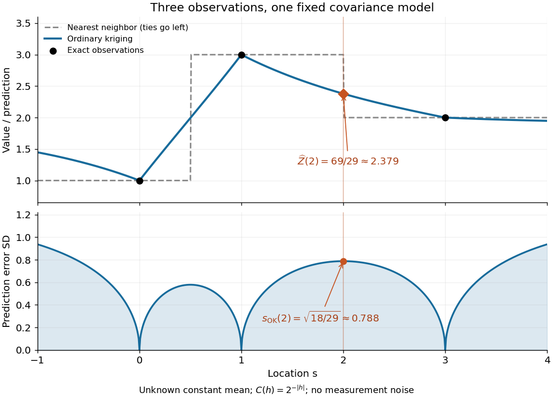
Ordinary kriging combines three samples and reports uncertainty under a fixed exponential covariance model
. Details. The upper panel applies the same ordinary kriging calculation at each target location. The lower panel shows the square root of its error variance, in the units of the observations. It is zero at the exact observation locations and rises between and beyond them. No confidence interval is inferred from a variance alone; a probability distribution assumption is needed to attach a coverage level.
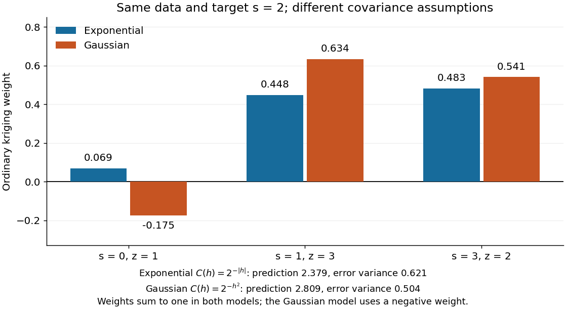
The weights are not required to be positive. Keep the same observations and target, but replace the covariogram by the smoother Gaussian kernel . ThenThe negative coefficient compensates for dependence between samples; the constraint eliminating bias still holds. Kriging is not generally a convex combination, and its prediction need not stay between the observed values. A smaller model-based error variance does not establish that one covariance function is better supported by these three observations.


Universal kriging allows an unknown regression drift:The design matrix has full column rank, its entries and are known, and the regression coefficients are unknown. For example, rows and target row allow a linear spatial trend. Requiring to have zero bias for every gives . With known positive-definite matrix observation covariance matrix , the minimizing weights solvewhere is a vector of Lagrange multipliers. Equivalently, the generalized least squares estimate and prediction areThe first term is the estimated trend alone; the second predicts the correlated regression residuals. With , the error variance isThe last, nonnegative term accounts for estimating the specified drift coefficients. Merely inserting a fitted drift into simple kriging and keeping its known-mean error variance would omit this term. For a Gaussian random field, the same expressions arise by integrating over drift coefficients in a diffuse prior distribution limit; this is an additional inferential interpretation, not an assumption required by the linear optimization.[ref]
Gaussian Processes for Machine Learning by Carl Edward Rasmussen and Christopher K. I. Williams. §2.7, pp. 27–28, equations (2.38)–(2.42)
Decay of autocorrelation implies weak convergence of an observable by Codex 0 Created 2026-10-05 Updated 2026-10-06
Codex 0 Created 2026-10-05 Updated 2026-10-06For a probability measure-preserving system, if , then converges weakly in to . Centre ; its autocorrelations tend to zero. The isometry identity gives the same decay against each , hence by approximation against their closed forward span. Against its orthogonal complement the correlations are exactly zero. Orthogonal decomposition by a closed subspace finishes the proof without invertibility.
The kinetic helicity conservation law impliesTherefore is materially constant exactly when the right side vanishes. Incompressible flow together with constancy of along vortex lines is sufficient. In compressible flow, the density-normalized quantity satisfies .
For the unscaled objective , the kernel-ridge hat matrix is . Its prediction variance is . For eigenvalues , use and to bound the variance and the squared bias. The latter also uses the reproducing property and Bessel inequality, and does not require invertibility of .
EXISTING BODY EXPANSION, not a new concept: replace the present one-direction definition of Faithfulness of a directed acyclic graph in probability-and-statistics.bigb, under Causal directed acyclic graph, with the following body. Retain its existing header and parent.
A horizontal-velocity perturbation depending only on height has zero vertical velocity for nonzero wavenumber under incompressibility. Its pressure amplitude then vanishes in the unstratified vertical momentum equation.
An adverse radial specific entropy gradient can drive an oscillatory instability through the finite lag supplied by thermal conduction or relaxation. This differs from a viscous-convective instability, in which viscosity changes rotational stabilization.
For a positive inner magnetic torque , define . Integrating steady conservation of angular momentum gives . With Keplerian rotation, this determines the surface density of a disk in the displayed formula.
K-theory of the sphere bundle of copies of a complexified real tautological line by Codex 0 2026-10-05
Codex 0 2026-10-05Let be the complexification of a real vector bundle of the tautological bundle over Real projective space . For , the K-theory Euler class of is , andThe K-theory Gysin sequence of a sphere bundle gives an extension by , which splits as an exact sequence of abelian groups.
MIRI's low-resolution spectroscopy includes a slitless time-series mode for exoplanet observations. Its useful coverage includes the – region, with longer-wavelength limits dependent on calibration and sensitivity. See the instrument guide.
The NIRISS single-object slitless spectroscopy mode measures time-series spectra from to . It supports exoplanet transmission spectra and eclipse observations, as described in the instrument guide.
There are unlisted articles, also show them or only show them.