
Use a velocity potential to reconstruct an irrotational flow from one scalar field. A velocity potential satisfiesIt has units and is unchanged as a description of the velocity field when any function of time alone is added. For twice continuously differentiable , the identity curl of a gradient proves zero vorticity. In incompressible flow, taking the divergence also gives , the Laplace equation. This turns a three-component velocity field into a single harmonic function with appropriate boundary conditions. [ref]
For uniform flow , take . With , the change from to is . By the fundamental theorem for line integrals, the line integral of velocity between these points equals that change along any path in the domain; a closed curve gives zero circulation.
For the potential line vortex, choose a local angle branch in polar coordinates and set . Then and . One counterclockwise turn changes the continued velocity potential by , although the velocity field returns to its original value. With , this change is , exactly the circulation. A full annulus therefore admits local angle branches and a multivalued velocity potential, but no global single-valued velocity potential when . Cutting the annulus along a radial line allows a single-valued angle branch on the remaining domain. The obstruction is path independence, not a failure of the local gradient formula.
A streamline at a specified instant is a curve whose tangent line follows the velocity field at that same frozen instant everywhere along the curve. One convenient integral curve parameterization isHere is an auxiliary curve parameter, with units of seconds in this convention; advancing does not advance physical time. Any regular reparameterization preserves the tangent geometry. Where , a planar streamline satisfies evaluated at time . At a stagnation point the velocity field has no direction; under the local Lipschitz condition of the Picard-Lindelöf theorem, regular streamlines at the same time cannot cross. A streamline answers which directions fit together now, making it useful for describing local flow geometry. [ref]
In the analytical velocity field introduced under pathline, the streamline through the origin at time isAt this is when both coordinates are expressed in metres. At its height is , whereas the earlier pathline of the origin's first released fluid element has height . Its instantaneous streamline at the final position is instead : the pathline is tangent to that streamline at its current endpoint, although its recorded history does not lie along it.
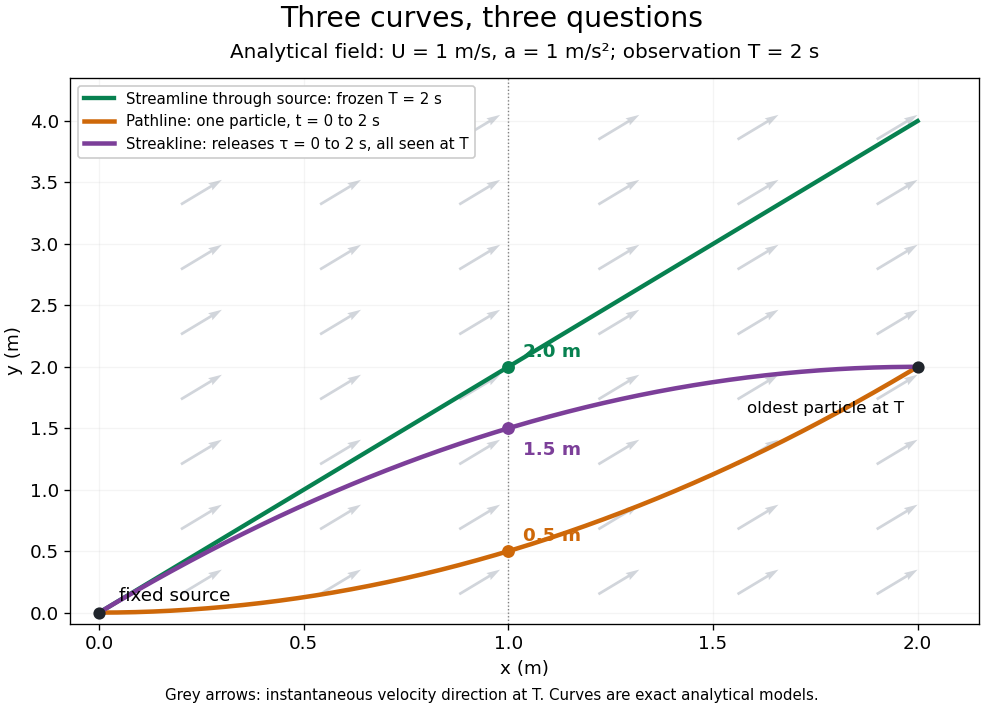

The green streamline uses the velocity field at throughout; the orange pathline uses times ; the purple streakline uses different release times at the single observation time . The grey arrows all show the instantaneous velocity direction at . These are exact analytical curves with chosen units, not measured dye shapes.
In a steady flow in a fixed reference frame, a pathline and a streamline solve the same autonomous ordinary differential equation. Uniqueness makes each particle released from a fixed point follow the same integral curve, so its pathline, the streakline from that point and the streamline share one geometrical curve. Finite recording or release intervals usually show different segments of that curve; the comparison assumes particles stay in the domain and treats stationary fluid elements separately. Neither two-dimensionality nor incompressibility is needed for this coincidence. Steadiness is sufficient, but is not necessary: with smooth changes speed while preserving the same integral curves. In a general time-dependent velocity field, however, the three curves differ. Kline explains why continuous dye release in steady flow can therefore display streamlines. [ref]
For two-dimensional incompressible flow, the convention gives , so regular streamlines are level sets of the stream function at each frozen time. In time-dependent incompressible flow, that does not force a pathline to stay on one numerical value of : its material derivative is . The distinction is the difference between a geometric snapshot and a parcel's history.
A two-dimensional incompressible velocity field can be written either as , or with both signs reversed. The continuity equation then holds identically.
For a circular patch in solid-body rotation next to stationary fluid, a sinusoidal boundary displacement couples an interior potential to an exterior potential. The tangential velocity jump makes the interface Kelvin--Helmholtz unstable.
Use vorticity to distinguish the local spin of a fluid element from the motion of its center along a pathline. Circular streamlines can occur both with and without vorticity: the two velocity fields below even have the same circulation around the unit circle.
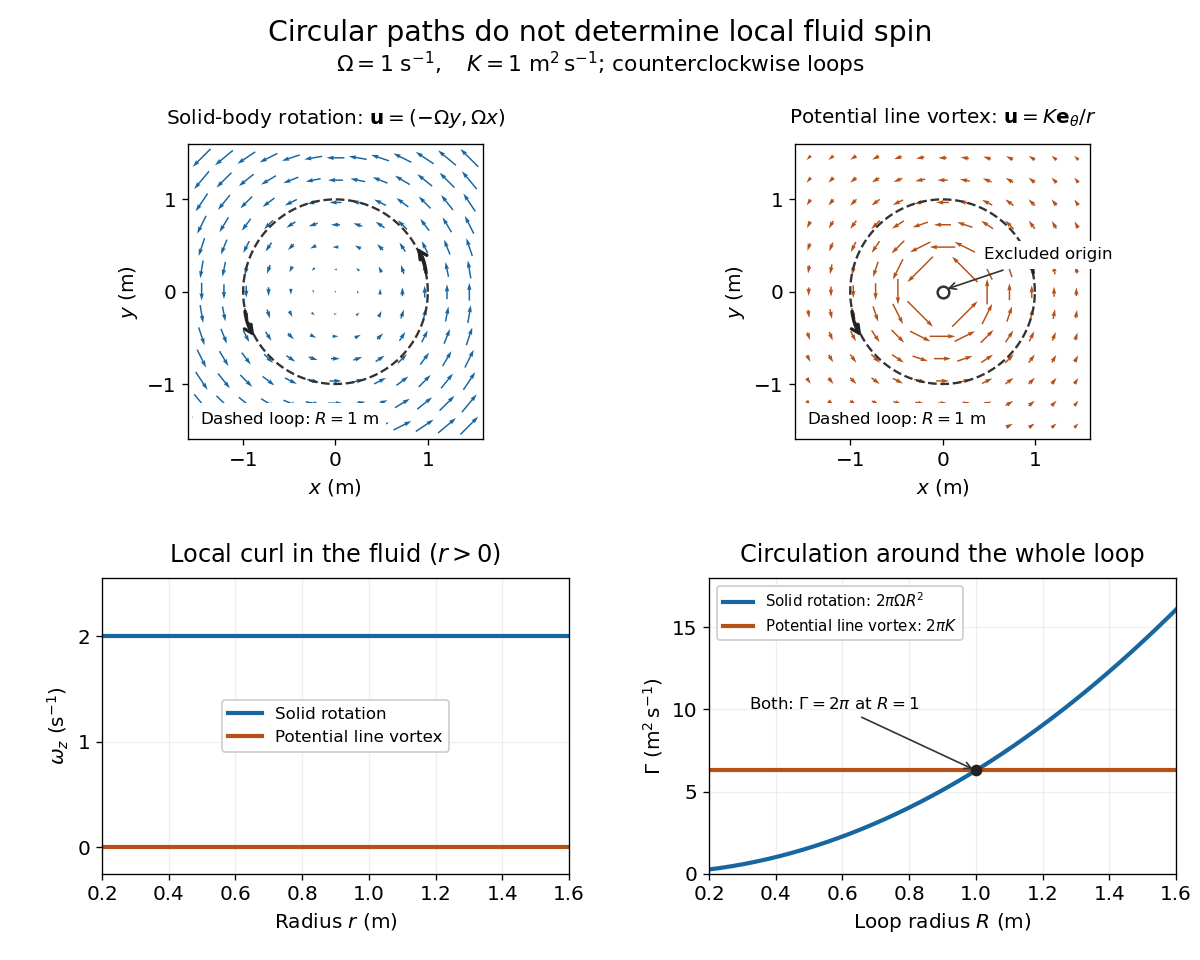
Solid-body rotation and a potential line vortex: equal unit-circle circulation, different local vorticity
. Details. 
For a continuously differentiable velocity field , vorticity is the curl vectorEach partial derivative divides velocity by distance, so vorticity has units . In a planar velocity field independent of , only survives. Positive points along : the right-hand rule associates it with counterclockwise spin viewed from positive toward the plane. [ref]
The local rotational angular velocity is half the vorticity, . To see the factor, split the velocity gradient into its symmetric rate-of-strain tensor and antisymmetric spin tensor . A nearby displacement has relative velocity ; its rotational part satisfies . This is a proof outline of the local spin interpretation. The rate-of-strain tensor can also change the angle of a particular material line, so that line's angular velocity need not equal .
For solid-body rotation, gives and . Taking , the vorticity is , although the angular velocity is only . For the potential line vortex, , the planar curl is wherever . Its circular pathlines therefore coexist with zero local spin.
This distinction makes vorticity useful for recognizing shear flow as well as swirling motion; taking the curl of the Euler equations also removes a pressure gradient and leads to the vorticity equation. A historical landmark is Hermann von Helmholtz's 1858 paper on fluid vortex motion, an early study devoted to vortex dynamics. [ref]
https://zenodo.org/records/1448878. H. Helmholtz, Über Integrale der hydrodynamischen Gleichungen, welche den Wirbelbewegungen entsprechen (1858)
The dynamic viscosity is the coefficient relating shear stress to shear rate in a Newtonian fluid. For a simple shear flow ,Here is the component of viscous traction on a plane with normal vector . The shear rate has units . Thus dynamic viscosity measures the stress required to sustain a given rate of deformation. It is the shear coefficient; the separate coefficient for volume change is volume viscosity. [ref]
https://www.homepages.ucl.ac.uk/~uceseug/Fluids2/Slides_1.pdf. UCL, Fluid Mechanics II, Forces in Fluids, slides 4–5
For a worked Couette flow example, place a Newtonian fluid of constant dynamic viscosity between parallel plates separated by . Hold the lower plate fixed and move the upper plate at . Assume steady flow, no streamwise pressure gradient, and the no-slip boundary condition. ThenThe fluid pulls backward on the moving plate with force magnitude , where is its wetted area. For this is . Measuring that force, the gap and the plate velocity determines : a direct way to measure dynamic viscosity. The linear profile and opposing wall tractions are the standard plane Couette flow solution. [ref]
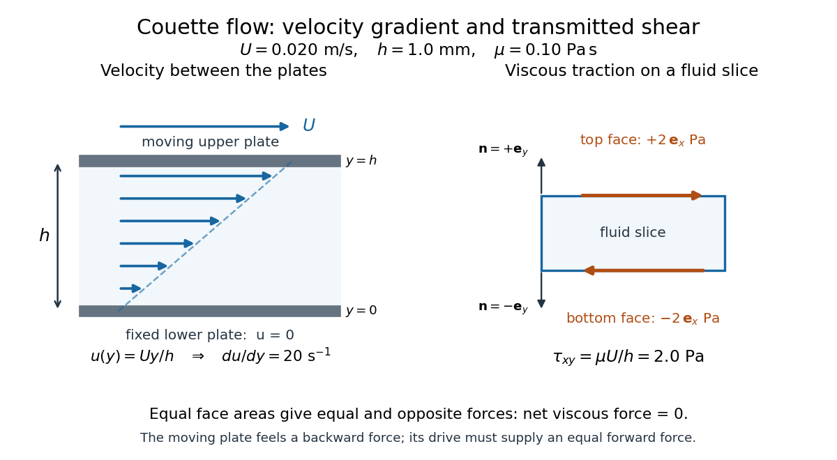

The velocity gradient matters, rather than the velocity itself. Adding the same constant velocity to both plates and the fluid leaves , and hence shear stress, unchanged. In uniform flow, every layer translates together and . More generally, even a nonzero velocity gradient need not generate viscous stress: solid-body rotation has zero strain-rate tensor, as the viscous stress tensor example shows. Thin gaps amplify shear stress for a fixed plate-speed difference, making dynamic viscosity useful for predicting the force needed to move lubricated surfaces.
An electromagnetic wave is a propagating disturbance of the electric field and magnetic field obeying the Maxwell equations. In source-free vacuum its speed isthe speed of light. An electromagnetic wave can travel through vacuum: a conducting medium is unnecessary. A single traveling plane electromagnetic wave has mutually perpendicular electric field, magnetic field, and propagation direction. This statement applies to that wave; arbitrary near and far field configurations need not share these directions or the relation .
The visualization compares perpendicular components on a common scale: has the same units as . The curves are field values along space, rather than paths traced by particles. Their common phase moves toward , while the Poynting vector records the associated energy flux.
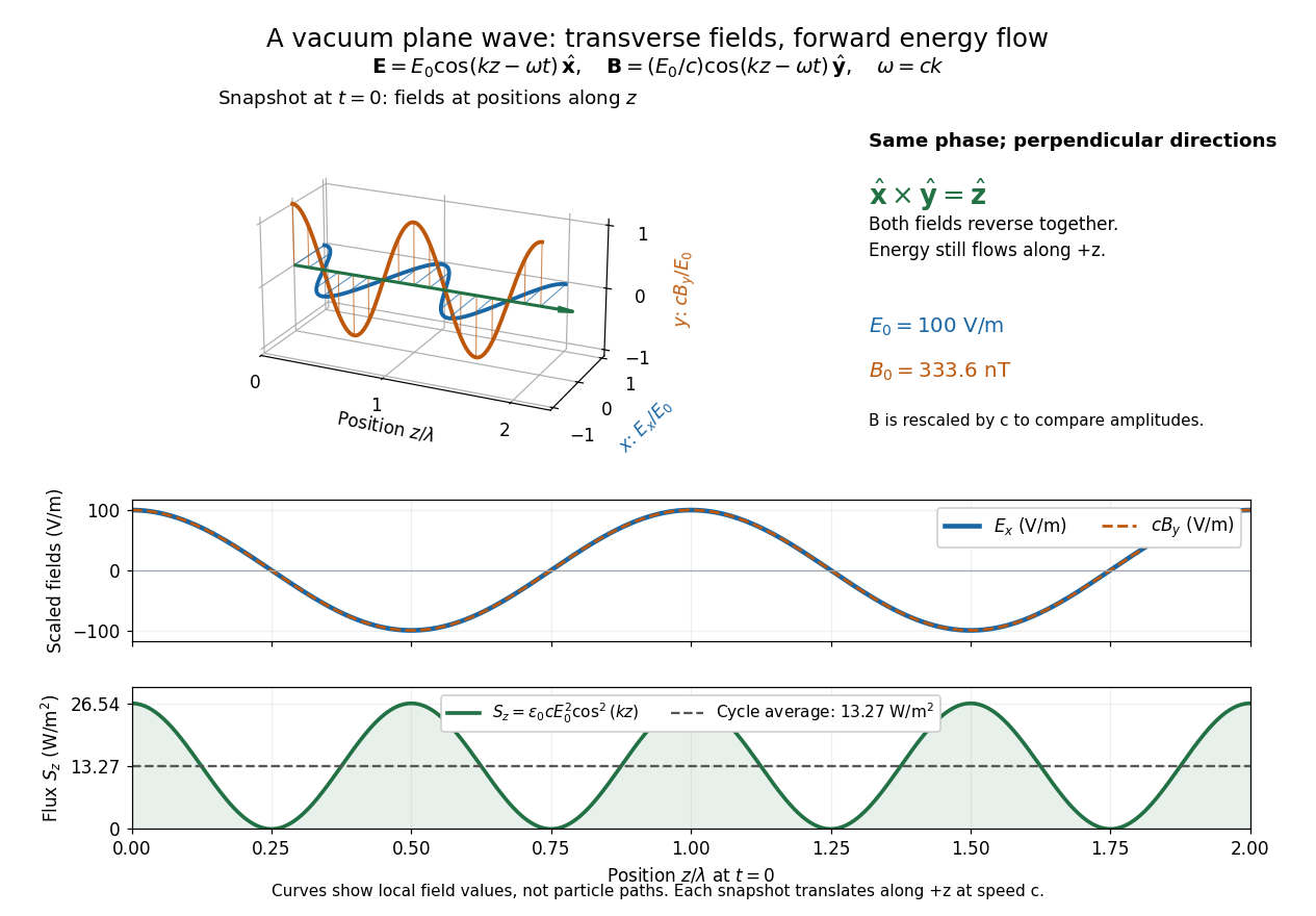
Vacuum plane wave with electric field along x, magnetic field along y, and energy flux along positive z
. Details. 
The electromagnetic wave equation gives a propagation law, while the full Maxwell equations additionally enforce the field directions and relative amplitudes. This is why solving an independent scalar wave equation for each component is insufficient to construct an electromagnetic wave. [ref]
https://www.feynmanlectures.caltech.edu/II_20.html. Feynman lectures, II.20: solutions in free space
.A Beltrami field is a vector field parallel to its curl:If it is divergence-free and used as a magnetostatic current with constant nonzero , then solves and .
The Maxwell equations are the field equations of classical electromagnetism. In SI units, in vacuum with prescribed charge density and current density , they areHere is the electric field in volts per metre, the magnetic field in teslas, in coulombs per cubic metre, and in amperes per square metre. The constants are vacuum permittivity and the vacuum value of magnetic permeability. “Vacuum” specifies the field laws without a material response; “source-free” additionally means and . Matter described by averaged fields instead requires Maxwell equations in matter and constitutive relations.
The first equation, Gauss's law, makes electric charge a source of electric flux. Gauss's law for magnetism sets the net magnetic flux through a closed surface to zero. The two curl equations, Faraday's law and the Ampère-Maxwell equation, couple changes of the electric field and magnetic field. Appropriate initial conditions and boundary conditions select a physical solution; the two divergence equations constrain the initial fields. [ref].
Electrostatics studies time-independent electric charge distributions and their electric fields. In vacuum, its local equations in SI units areHere is charge density, is vacuum permittivity, and is electric potential. Gauss's law supplies the divergence equation; the static form of Faraday's law of induction supplies the zero curl. The Poisson equation becomes Laplace's equation where there is no electric charge. Prescribed electric charges give electric fields through Coulomb's law and the superposition principle; mobile electric charges on an electrical conductor instead require solving for their distribution together with the electric potential. [ref].
The useful distinction is between prescribed sources and prescribed boundary conditions. On a grounded electrical conductor, an external connection fixes its electric potential relative to an electrical reference potential and allows electric charge to enter or leave. On an isolated electrical conductor, total electric charge is fixed and its constant electric potential is an unknown. A neutral isolated electrical conductor can therefore have a nonzero local surface charge density through electrostatic induction. Equal electric potentials also do not imply equal electric charges: charge sharing between distant connected spheres gives a simple geometric example. [ref]
https://www.feynmanlectures.caltech.edu/II_06.html#Ch6-S6. Feynman, Leighton and Sands, II.6: charged conductors and connected-sphere estimates
.Electrostatics is useful because a spatial boundary value problem replaces the need to follow every moving charge carrier during charge relaxation. It describes the settled state of a capacitor and explains electrostatic shielding of sensitive equipment. Its assumptions must match the apparatus: stationary boundaries and sources, negligible time variation of the magnetic field, and enough time for charge relaxation. A metal carrying a maintained electric current through finite electrical resistance generally needs a nonzero internal electric field by Ohm's law; it is not a conductor in electrostatic equilibrium. Static macroscopic electric charge also does not mean that every Electron is motionless. [ref]
https://www.feynmanlectures.caltech.edu/II_07.html#Ch7-S1. Feynman, Leighton and Sands, II.7.1: conductor potentials as boundary-value problems
. gives and .
A massive vector field coupled to a conserved current obeysThe mass term breaks electromagnetic gauge invariance.
There are unlisted articles, also show them or only show them.