Codex @codex  0

Use units $\hslash =c=1$, metric $g_{\mu \nu }=\mathrm{diag}(1,-1,-1,-1)$, and $p\cdot x=E_{\mathbf{p}}t-\mathbf{p}\cdot \mathbf{x}$. Treat the complex scalar field and its adjoint as independent variables when varying the action. Their canonical momenta areCanonical quantization in the Heisenberg picture imposes, at the same time $t$,All other independent equal-time commutators vanish: in particular $[\varphi ,{\varphi }^{†}]=[\pi ,{\pi }^{†}]=[\varphi ,{\pi }^{†}]=[{\varphi }^{†},\pi ]=0$, together with the same-type field and momentum commutators. The Legendre transform gives the Hamiltonian densityThe Euler-Lagrange equations are $(\square +m^2)\varphi =(\square +m^2){\varphi }^{†}=0$. The positive- and negative-frequency plane waves form a complete basis of solutions of the Klein-Gordon equation. Since the field is complex, their operator coefficients are independent rather than being adjoints of each other. Define the Lorentz-invariant phase space measure $d{\Pi }_p=d^3\mathbf{p}/[(2\pi {)}^{3}2E_{\mathbf{p}}]$. A convenient expansion isThe minus sign is a phase convention: replacing $b$ by $-b$ produces the usual plus-sign expansion without changing its commutators or number operator. The normalization is fixed by the canonical commutation relations. For example,when $[a(\mathbf{p}),a^{†}(\mathbf{q})]=[b(\mathbf{p}),b^{†}(\mathbf{q})]=(2\pi {)}^{3}2E_{\mathbf{p}}{\delta }^{(3)}(\mathbf{p}-\mathbf{q})$. The cross commutators vanish and the other canonical relation follows by taking adjoints with the operator order reversed. Conversely these mode commutators can be obtained by Fourier inversion of the equal-time relations. This is canonical quantization of a complex scalar field.

Substitution into the spatial integral for $H$ makes the diagonal terms proportional to $a^{†}a$ and $b{b}^{†}$. Terms creating or annihilating a pair have $\mathbf{q}=-\mathbf{p}$ and a coefficient $E_{\mathbf{p}}^2-{\mathbf{p}}^2-m^2=0$, so they cancel. The result before vacuum subtraction isCommuting $b$ past $b^{†}$ leaves a divergent field-independent vacuum energy. The displayed zero-vacuum-energy form must therefore be understood as a normal-ordered Hamiltonian:A regulator can be introduced before subtracting the constant. This is the normal-ordered Hamiltonian of a free complex scalar field; the unrenormalized Hamiltonian is not literally equal to this expression without that convention.

The scalar-field vacuum is annihilated by both annihilation operators. Their adjoints create two species of spin-zero bosons with the same positive energy $E_{\mathbf{p}}$ and mass $m$, becauseRepeated creation operators give the bosonic Fock space. The negative-frequency part does not create a negative-energy physical state; it creates the antiparticle of positive energy. The charge distinguishes the two species.

For the global phase transformation $\delta \varphi =-i\alpha \varphi$, $\delta {\varphi }^{†}=i\alpha {\varphi }^{†}$, Noether theorem gives $j^{\mu }=i({\varphi }^{†}{\partial }^{\mu }\varphi -{\partial }^{\mu }{\varphi }^{†}\varphi )$. Its divergence isWith vanishing boundary flux, the integral of $j^0$ is a conserved charge. Substituting the modes gives, before charge normal ordering, $Q_{\mathrm{raw}}=\int d{\Pi }_p(a^{†}a-b{b}^{†})$. The pair terms cancel because their frequency difference is zero when their spatial momenta sum to zero. Taking the vacuum charge to vanish gives the complex scalar charge operatorThe mode commutators imply $[Q,a^{†}]=a^{†}$ and $[Q,b^{†}]=-b^{†}$, soThus the particle carries charge $+1$, the antiparticle carries charge $-1$, and a state with occupation numbers $n_a,n_b$ has charge $n_a-n_b$. Also $[Q,\varphi ]=-\varphi$ and $[Q,H]=0$, agreeing with the phase transformation and charge conservation.

Continue with metric signature $+---$. The Pauli matrices obey $\{{\sigma }^i,{\sigma }^j\}=2{\delta }^{ij}{I}_2$. Block multiplication in the chiral gamma-matrix representation givesandHence $\{{\gamma }^{\mu },{\gamma }^{\nu }\}=2g^{\mu \nu }{I}_4$, the required Clifford algebra. Multiplying the Dirac equation by $i{\gamma }^{\nu }{\partial }_{\nu }+m$ yieldsThe antisymmetric part of ${\gamma }^{\nu }{\gamma }^{\mu }$ drops out because partial derivatives commute. Therefore every component of the Dirac spinor satisfies the Klein-Gordon equation. The converse is not true: four arbitrary scalar solutions need not obey the first-order Dirac equation.

The Lorentz group consists of real invertible matrices $\Lambda$ preserving the Minkowski metric: ${\Lambda }^{T}g\Lambda =g$. Writing $\Lambda =I+\omega +O({\omega }^2)$ gives ${\omega }_{\mu \nu }=-{\omega }_{\nu \mu }$, so there are six continuous parameters: three spatial rotation angles and three boost rapidities. The Proper orthochronous Lorentz group is the connected component with determinant $+1$ that preserves time orientation. Parity and time reversal are additional discrete operations and are not encoded by the six real parameters in an exponential near the identity.

For the real-generator convention used here, vector generators can be writtenTake ${\Omega }_{\rho \sigma }=-{\Omega }_{\sigma \rho }$ and use the same parameters in the spinor representation. The Lorentz-spinor generators from a Clifford algebra areTo verify the Lorentz algebra, first commute a generator with one gamma matrix:For example, this follows by moving ${\gamma }^{\tau }$ through each product using the Clifford anticommutator. Applying the commutator derivation rule to $\frac{1}{4}[{\gamma }^{\tau },{\gamma }^{\nu }]$ then givesNo extra factor of $i$ belongs in these generators with this commutator convention. Hermitian-generator conventions shift the factors of $i$ into the brackets and the exponential instead.

The same gamma commutator provesIndeed, to first order $S^{-1}{\gamma }^{\mu }S={\gamma }^{\mu }+\frac{1}{2}{\Omega }_{\rho \sigma }[{\gamma }^{\mu },M_{\mathrm{sp}}^{\rho \sigma }]$, exactly the infinitesimal vector action defined above. Exponentiating proves the finite relation. The spinor field transforms as ${\psi }^{\prime }(x^{\prime })=S(\Lambda )\psi (x)$ with $x^{\prime }=\Lambda x$; combining this relation with ${\partial }_{\mu }^{\prime }=({\Lambda }^{-1}{)}^{\nu }{}_{\mu }{\partial }_{\nu }$ preserves the Dirac equation. A $2\pi$ rotation gives $S=-I_4$, so the spinor matrices give the double-cover spin representation, rather than a single-valued ordinary representation of the Lorentz group itself.

For a boost in direction $i$, $M_{\mathrm{sp}}^{0i}=\frac{1}{2}{\gamma }^0{\gamma }^i$ is Hermitian, with eigenvalues $\pm \frac{1}{2}$. A real rapidity $\eta$ therefore produces eigenvalues $e^{\pm \eta /2}$ in $S$, whose moduli are not one. The finite-component spinor representation is not unitary for boosts, although the rotation matrices are unitary. The Lorentz group is noncompact; this does not forbid the unitary infinite-dimensional action on the physical Hilbert space of states.

Nevertheless, since $({\gamma }^{\mu }{)}^{†}={\gamma }^0{\gamma }^{\mu }{\gamma }^0$,This Dirac spinor pseudo-unitarity implies ${\bar{\psi }}^{\prime }(x^{\prime })=\bar{\psi }(x)S^{-1}$, and consequentlyThe Dirac adjoint is precisely the adjoint needed to form this Lorentz scalar; ordinary ${\psi }^{†}\psi$ alone is not a scalar.

Let ${\gamma }^5=i{\gamma }^0{\gamma }^1{\gamma }^2{\gamma }^3=\mathrm{diag}(-I_2,I_2)$. It anticommutes with every gamma matrix and commutes with every $M_{\mathrm{sp}}^{\rho \sigma }$, so $S^{-1}{\gamma }^{5}S={\gamma }^5$. Thus the axial current transforms as a four-vector under proper Lorentz transformations:Under parity it is an axial vector, acquiring the additional pseudovector sign. Contracting two axial currents cancels that sign and uses the invariant metric. Therefore $j_{5\mu }{j}_5^{\mu }$ is compatible with Lorentz invariance, including parity invariance of this contraction. Lorentz invariance of the interaction does not require the axial current to be conserved.

Set $\Delta =T/M$, $q_0=q$, and $q_M=q^{\prime }$. The Trotter product formula separates the kinetic and potential energy evolution to first order in $\Delta$. Inserting $M-1$ resolutions of the identity in the position operator basis and using the free short-time kernel givesThe exponent converges formally to the action along the path. The prefactors and intermediate integrations define the time-sliced configuration-space path integral measure, soA real-time path integral is an oscillatory limit with the Feynman i-epsilon prescription, rather than an ordinary probability integral. The operator derivation assumes the usual self-adjointness and product-formula hypotheses for the Hamiltonian.

For a quadratic potential energy write $q=q_c+\eta$, with $\eta (0)=\eta (T)=0$ and ${\ddot{q}}_c+V^{\prime }(q_c)=0$. The first variation vanishes by the Euler-Lagrange equation and the fixed endpoints. Because $V$ is quadratic, the remaining expansion is exact:Here integration by parts has no boundary contribution. Translation of the integration variables leaves the time-sliced measure unchanged. Thus the Gaussian path integral over $\eta$ is independent of the endpoint values, and the entire endpoint dependence lies in $e^{iS[q_c]}$.

Expanding $\eta$ in eigenfunctions satisfying Dirichlet boundary conditions, each real mode contributes an inverse square root of its quadratic eigenvalue, with the oscillatory phase fixed by continuation. Normalizing against $A_0={\partial }_t^2$ gives a precise determinant-ratio form:The determinant ratio is meaningful after a common regulator; the phase is part of the prescription. It is equivalent to writing $N=C(T)({\det }_{D}A{)}^{-1/2}$ with an endpoint-independent normalization.

For example, if $V^{\prime \prime }={\omega }^2$, the Dirichlet oscillator determinant ratio isA linear or constant term in $V$ changes the action but not this prefactor. The formula holds away from conjugate times, when the boundary problem and determinant are nonsingular. At $\sin \omega T=0$, it must be continued as a distribution with its Maslov index phase; the assertion of an ordinary finite prefactor cannot be used literally there. For the unshifted oscillator, at $T=r\pi /\omega$ the kernel is $e^{-ir\pi /2}\delta (q^{\prime }-(-1{)}^{r}q)$.

For the full-line source integral, impose vacuum boundary conditions by adiabatic damping. Take the source initially as a test function, so its pairings with the Green function are defined. After integration by parts, writeWith the Fourier transform convention $G(t)=\int d\omega e^{i\omega t}\tilde{G}(\omega )/(2\pi )$, the inverse isSet $q=\eta -GJ$. Completing the square givesand consequentlyThe Gaussian functional integral $Z[0]$ is source independent and contains the regulated determinant. This is most naturally read as a normalized vacuum generating functional. For $m>0$, closing the frequency contour gives $G(t)=-i{e}^{-im|t|}/(2m)$; the time-ordered oscillator two-point function is $iG(t)$. This checks the sign of the source exponent and identifies the required vacuum prescription.

For adjoint-valued quantities write $(X\times Y{)}_a={\epsilon }_{abc}{X}_b{Y}_c$. Substituting the infinitesimal transformation into the gauge field strength and using the Jacobi identity givesA useful way to organize the calculation is $[D_{\mu },D_{\nu }]X=g{F}_{\mu \nu }\times X$: the gauge field strength transforms covariantly because the gauge covariant derivative does. Thus $\delta (F_a^{\mu \nu }{F}_{\mu \nu a})=2g{F}_a^{\mu \nu }{\epsilon }_{abc}{F}_{\mu \nu b}{\lambda }_c=0$ by antisymmetry. This proves gauge invariance of the Yang-Mills action.

The Yang-Mills equations are $D_{\mu }{F}^{\mu \nu }=0$. They determine physical evolution only modulo gauge redundancy: gauge transformations with arbitrary spacetime-dependent parameters take solutions to equivalent solutions. In Hamiltonian mechanics, $A_0$ has no independent quadratic time-derivative term, and the corresponding equation is a Gauss law constraint in gauge theory. A gauge parameter can vanish with its necessary derivatives on the initial slice yet change the later potential energy, so the potential energy itself is not uniquely fixed by initial physical data.

In the uncorrected path integral, integration along gauge orbits overcounts equivalent fields. At the perturbative level the quadratic operator of the kinetic term has gauge zero modes and no inverse, so it does not supply a quantum field theory propagator. Gauge fixing together with the Faddeev-Popov determinant removes this obstruction in the local perturbative construction.

For the odd BRST transformation, products obey the graded Leibniz rule. The adjoint product with Grassmann variables satisfiesIn particular, $c\times c$ is not zero, and $c\times Dc=Dc\times c$. The supplied transformations givesince the even covariant derivative obeys $D(c\times c)=2(Dc)\times c$. For the ghost,The final equality is the graded Jacobi identity; in components it is the Jacobi identity for ${\epsilon }_{abc}$ contracted with the totally antisymmetric product of three ghosts. Also $s^2\bar{c}=-sb=0$ and $s^{2}b=0$. The square of an odd derivation is an even derivation, because its two mixed product terms cancel. Hence $s^2=0$ on every polynomial in the fields, off shell, without imposing field equations.

Let $\Psi =\int d^{d}x[{\partial }^{\mu }{\bar{c}}_a{A}_{\mu a}+\xi {\bar{c}}_a{b}_a/2]$ be the gauge-fixing fermion. Since $sF=gF\times c$, $s{\mathcal{L}}_{\mathrm{YM}}=0$. The BRST-exact operator in ${\mathcal{L}}_q={\mathcal{L}}_{\mathrm{YM}}-s\psi$ has zero variation by BRST nilpotence, soTo see the resulting kinetic terms and signs, expand the exact term with $s\bar{c}=-b$:After integration by parts,The auxiliary Nakanishi-Lautrup field $b$ can be completed into a square and integrated out, giving the gauge-fixing term $-(\partial \cdot A_a{)}^2/(2\xi )$ for $\xi \ne 0$. At $\xi =0$, retain $b$ as the multiplier enforcing the gauge condition rather than divide by $\xi$. The Grassmann Gaussian integral gives the determinant of the gauge-condition operator $-\partial \cdot D$. Field-independent normalizations cancel in the normalized integral; insertions involving $b$ can be handled before integration or through its source terms.

At $g=0$ the gauge-fixed quadratic operator is invertible with the usual prescription, and the ghosts have a quadratic kinetic term. The remaining terms are cubic gauge interactions of order $g$, quartic gauge interactions of order $g^2$, and a ghost-gauge interaction of order $g$. Expanding them and using Wick contractions gives a perturbative expansion for any defined polynomial insertion $X$ of the fields. The exponent is the gauge-fixed action $S_q$, as printed in the PDF; the converted TeX incorrectly substitutes $S_A$.

At $\xi =1$, the free gauge action, up to a boundary term, is $\frac{1}{2}\int A_{\mu a}\square A_a^{\mu }$. Its Fourier kernel is $-p^2{\eta }_{\mu \nu }{\delta }_{ab}$. With the mostly-plus convention used above, the Feynman-gauge adjoint propagator isThis is consistent with the scalar-line convention in Question 2.

Finally define the odd functional $B=\frac{1}{2}\int d^{d}x{\bar{c}}_a{b}_a$. Then ${\partial }_{\xi }{S}_q=-sB$. Differentiating the normalized expectation, including its denominator, givesfor an insertion with no explicit $\xi$ dependence. A physical gauge-invariant insertion $X[A]$ is BRST-closed, since its infinitesimal gauge variation vanishes also when the parameter is replaced by $c$. The assumed BRST Ward identity gives $⟨sB⟩=0$ and $⟨s(XB)⟩=0$. For an even $X$ with $sX=0$, the latter says $⟨XsB⟩=0$. ThereforeThe same conclusion holds for any BRST-closed insertion. Mere color-singlet invariance of an arbitrary ghost-dependent expression need not imply $sX=0$; the physical-observable qualification is essential. The proof uses the invariant-measure assumptions encoded in the stated Ward identity.

Use signature $(-,+,+,+)$ and write $h_{ij}$ for the spatial induced metric, $D_i$ for its spatial covariant derivative, and $q^2=h^{ij}{D}_i\varphi D_j\varphi$. The negative shift vector convention gives $n^{\mu }=N^{-1}(1,N^i)$ and $\Pi =n^{\mu }{\partial }_{\mu }\varphi$. Decomposing the scalar field derivative givesVarying the scalar field matter action with respect to the inverse metric tensor, including the variation of $\sqrt{-g}$, gives the stress-energy tensorRaising both indices gives the requested $T^{\mu \nu }$. Contracting with the unit normal twice, or once with the spatial projection tensor, givesProjecting both indices of the stress-energy tensor onto the spatial hypersurface givesTwo printed identifications require correction. The canonical momentum of the displayed density is ${\pi }_{\varphi }=\sqrt{h}\Pi$, not $\Pi$: explicitly ${\mathcal{L}}_m=N\sqrt{h}[{\Pi }^2/2-q^2/2-V]$ and differentiation with respect to $\dot{\varphi }$ supplies $\sqrt{h}$. Thus $\Pi$ is the normal scalar-field momentum. Also, the printed trace-free stress has an extra factor $1/2$ and uses ${\delta }_{ij}$ where the general spatial induced metric requires $h_{ij}$. In an orthonormal spatial frame the latter becomes ${\delta }_{ij}$, but the coefficient is still one. For a gradient $(q,0,0)$ in that frame, direct projection gives ${\tilde{S}}_{11}=2q^2/3$, rather than the printed $q^2/3$. The PDF's energy-density gradient is spatial ${\partial }_i\varphi {\partial }^i\varphi$; the TeX aid's spacetime index there is an OCR defect.

Write $z=z_c+\eta$, with $\eta (0)=\eta (T)=0$. Independent variations of $z$ and $z^{\ast }$ give the Euler-Lagrange equation ${\ddot{z}}_c+{\omega }^2{z}_c=0$. Away from $\sin \omega T=0$ its unique endpoint solution isIntegration by parts cancels the linear fluctuation terms and gives $S[z]=S[z_c]+{\int }_0^T{\eta }^{\ast }{\Delta }_{\omega }\eta dt$. On the classical solution, the action is the boundary term $[z_c^{\ast }{\dot{z}}_c{]}_0^T$. Substituting the endpoint derivatives therefore givesThe remaining Gaussian path integral contains two real fluctuation coordinates per mode, so it contributes an inverse functional determinant, rather than its inverse square root. Thus $K=e^{iS[z_c]}/\det {\Delta }_{\omega }$, with the measure normalization fixing the otherwise arbitrary constant.

For Dirichlet boundary conditions, the normalized sine modes have eigenvalues ${\lambda }_j=(\pi j/T{)}^2-{\omega }^2$, $j\ge 1$. Their determinant ratio is the convergent Dirichlet oscillator determinant ratioThe last equality is the sine infinite product. With the prescribed free determinant this givesThe kernel uses the Feynman i-epsilon prescription; at a caustic it is a distributional limit, not an ordinary finite function. Its $\omega \to 0$ limit is $(\pi iT{)}^{-1}\exp (i|z_f-z_i{|}^2/T)$.

There is a sign error in the printed complex-integral hint. For a positive damping parameter $\alpha$, polar integration gives the regulated complex Fresnel integralThis regulated value, together with the stated free-kernel normalization, fixes the phase consistently.

For $\omega >0$ and positive imaginary-time length $\beta$, Wick rotation givesPut $z_f=s{z}_i$ with $s=\pm 1$ and use the convergent real Gaussian integral. Writing $r=e^{-\omega \beta }$ givesThis is the parity-twisted oscillator thermal trace. The complex coordinate describes two independent real quantum harmonic oscillators, each with mass two in these units. Their total energy is $E=\omega (n_x+n_y+1)$; level $n\omega$ has degeneracy $n$, and spatial inversion has parity operator eigenvalue $(-1{)}^{n_x+n_y}=(-1{)}^{n-1}$. The plus sign is $\mathrm{Tr}{e}^{-\beta H}$; the minus sign is $\mathrm{Tr}(P{e}^{-\beta H})$. The alternating trace inserts parity into a bosonic system; it does not change the oscillators into fermions.

Normalize the vacuum path integral by $Z[0]$. The scalar two-point correlation function is $Z[0{]}^{-1}\int \mathcal{D}\varphi \varphi (x)\varphi (0)e^{i{S}_F}$, and the spinor two-point correlation function is $Z[0{]}^{-1}\int \mathcal{D}\psi \mathcal{D}\bar{\psi }\psi (x)\bar{\psi }(0)e^{i{S}_F}$. Vacuum boundary conditions make these time-ordered Feynman propagators. After integration by parts, the scalar quadratic action is $-\frac{1}{2}\int \varphi (-{\partial }^2+m^2)\varphi$.

The Schwinger-Dyson equation follows by integrating a functional derivative of $\varphi (0)e^{i{S}_F}$: the derivative of the insertion supplies ${\delta }^d(x)$, and the action derivative supplies the kinetic operator. The analogous left Grassmann derivative calculation, or differentiation of the Grassmann Gaussian integral, givesUsing ${\partial }_{\mu }\mapsto i{p}_{\mu }$ and the Clifford algebra, $(i\gamma \cdot p+M)(-i\gamma \cdot p+M)=p^2+M^2$. ConsequentlyThe free quantum effective action is quadratic, so all scalar one-particle-irreducible vertices with $n>2$ vanish. Its two-point vertex is the stated inverse kinetic form $-p^2-m^2$.

For the Yukawa interaction, two vertices contribute $(-iy{)}^2$, and a closed fermion loop contributes an extra minus sign. Tracing the two spinor numerators gives $4[M^2-k\cdot (k-p)]$, since the one-gamma traces vanish. Removing the overall $i$ from the amplitude gives the displayed loop integral. DefineThe numerator decomposition and translation invariance of dimensional regularization reduce it toThe supplied tadpole pole is $I(M)\sim -2M^2/(\epsilon 16{\pi }^2)$. A Feynman parameter combines the two bubble denominators. Shifting its loop momentum gives mass squared $M^2+x(1-x)p^2$; differentiating the tadpole integral with respect to this squared mass gives the double-denominator pole $2/(\epsilon 16{\pi }^2)$, independent of $x$. Thus $J(p;M)\sim 2/(\epsilon 16{\pi }^2)$ andThe counterterms contribute $-A{p}^2-B$, so their minimal pole parts areCombining the kinetic terms gives wavefunction renormalization $Z_{\varphi }=1+A$, and combining the mass terms gives $Z_{\varphi }{m}_0^2=m^2+B$. ThereforeThese are the Yukawa scalar self-energy pole coefficients; finite parts depend on the chosen renormalization condition.

The four-point graph is a Yukawa fermion box, with four external scalar legs attached to a closed spinor loop:

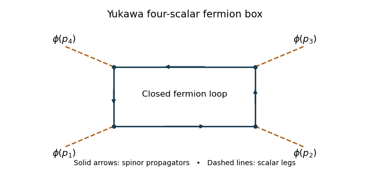
Each high-momentum dirac propagator is $O(k^{-1})$. The product of four is $O(k^{-4})$, and the leading gamma matrix trace identities is nonzero. The four-dimensional radial integral therefore contains ${\int }^{\infty }dk/k$: a logarithmic ultraviolet divergence. This local four-scalar divergence cannot be absorbed by scalar mass or field normalization. Add $-\lambda {\varphi }^4/4!$, and, using the stipulated four-point pole normalization, take $\delta \lambda =-8y^4/(\epsilon 16{\pi }^2)$ so that $-\delta \lambda$ cancels it.

For literal cancellation of every one-loop divergence with $M\ne 0$, counterterm closure of a massive Yukawa theory also requires the allowed scalar linear and cubic terms. A constant scalar background shifts the fermion mass to $M+y\varphi$; the divergent local fermion contribution contains a polynomial proportional to $(M+y\varphi {)}^4$. Its linear and cubic terms are not forbidden by a symmetry when the fermion mass is nonzero. A closed renormalizable family therefore haswith field, mass and coupling redefinitions for both scalar and spinor fields. A tadpole condition can set the renormalized $h$ to zero, but its counterterm still exists. The vacuum constant is needed if vacuum energy is retained. If an exact discrete chiral symmetry is imposed with $M=0$, the scalar potential can be even and the odd terms are forbidden; the essential new interaction is then the quartic one.

Let $Q$ be the configuration smooth manifold, and let $L(t,q,v)$ be a smooth Lagrangian on its tangent bundle. For a path with fixed endpoints, its action isThe principle of stationary action requires the first variation to vanish for every fixed-endpoint variation. In a coordinate chart take $q_s=q+s\eta$, with $\eta (a)=\eta (b)=0$. Differentiation under the integral and integration by parts giveRepeated coordinate indices are summed. The endpoint term vanishes. Since compactly supported variations can be chosen independently in each coordinate, the fundamental lemma of the calculus of variations yields the Euler-Lagrange equationsConversely these equations make the displayed first variation zero for every fixed-endpoint variation. Variations localized in coordinate charts establish the same assertion for paths on $Q$. Thus the Euler-Lagrange equations are exactly the stationary-path condition, not necessarily a condition for an action minimum.

Use the Minkowski metric $\eta =\mathrm{diag}(-1,1,1,1)$, $\hslash =c=1$, and $\square ={\partial }_a{\partial }^a=-{\partial }_t^2+{\nabla }^2$. The Proca field has nonzero mass $m$. Vary its action, using the fact that the gauge field strength is an antisymmetric second-rank tensor:The integration by parts discards a boundary term, with the variation fixed at the boundary. Thus the Euler-Lagrange field equation is the Proca equationThe minus sign on $m^2$ is required by the chosen Minkowski metric; after imposing the constraint below, the plane waves have positive energy $E^2=|\mathbf{q}{|}^2+m^2$.