
An acquisition duration from an exponential tail-energy tolerance chooses how long to continue recording when a validated optical-power envelope bounds the remaining energy. Suppose after time the true power satisfies , with and . The exponential-envelope tail-energy bound gives a remaining allowance after extension . For tolerance ,This is a conditional upper-bound calculation, not an inference from the last sample merely falling below a detector threshold.
An original uncertainty example has guaranteed parameter limits and . The remaining allowance increases with either parameter, so a tolerance requires . Using only best-fit values and would give about , which does not guarantee the same tolerance over the allowed set. Joint parameter constraints can tighten a bound, but their coverage must be justified.
In the positive-duration branch, the local sensitivities areThis acquisition-time sensitivity to tail-model parameters explains why an uncertain slow decay can matter more than a small amplitude correction. The derivatives change interpretation at the zero-duration boundary.
The envelope must apply to optical power throughout the unrecorded region. A later pulse or an unremoved persistent background can invalidate it. NIST's separate measurement of detector response illustrates why an electrical waveform's decay alone is insufficient.[ref]
Calibration Service for Low-level Pulsed-Laser Radiometers at 1.06 µm: Pulse Energy and Peak Power by Rodney W. Leonhardt. Appendix C.1–C.2, printed pp. 36–37
State the chosen time origin, tolerance units, valid envelope parameters and any other excluded intervals when reporting the acquisition requirement.An acquisition duration from a power-law tail-energy tolerance extends a measurement until the validated envelope's unrecorded energy is below a chosen tolerance. For the model in power-law tail from a decaying rate envelope, with ,The parent article integrates this envelope and inverts the tolerance. Writing , its positive-duration requirement is when ; otherwise no additional duration is required.
In applying the rule, uncertainty in the exponent can dominate the result. With fixed and , differentiating the active branch givesThe required duration decreases with a larger exponent. For a guaranteed parameter range, a validated lower bound on a power-law tail exponent is therefore more useful than its best-fit value alone. Since decreases with for every , using the smallest allowed exponent bounds the entire tail, not just one selected sample.
For an original design example, let , and . A nominal exponent gives initial allowance , and . If the validated exponent range is instead , its slowest permitted tail has initial allowance and requires . The nominal duration does not guarantee the tolerance over that range. Upper bounds on and can likewise be used conservatively because increasing either raises the envelope pointwise.
If the allowed exponents reach one or below, these envelope assumptions alone no longer supply a finite all-time energy guarantee. This is a limitation of the bound, not proof that the actual pulse has infinite energy. The model must also hold throughout the unobserved interval: later pulses, persistent backgrounds or an electrical detector tail misidentified as optical power can invalidate it. NIST's independent receiver-response measurement illustrates this last experimental distinction.[ref]
Calibration Service for Low-level Pulsed-Laser Radiometers at 1.06 µm: Pulse Energy and Peak Power by Rodney W. Leonhardt. Appendix C.1–C.2, printed pp. 36–37
The power-law examples are original conditional models, not observed decay laws attributed to that apparatus.Acquisition-time sensitivity to tail-model parameters measures how an inferred recording extension changes when the assumed optical tail changes. In the positive-duration branch of acquisition duration from an exponential tail-energy tolerance, writeHere bounds the initial tail power, is its decay time and the tolerated missed energy. Their first-order relative effects areThese logarithmic condition numbers of a tail-acquisition requirement distinguish a fractional amplitude error from a fractional decay-time error. For a stringent tolerance with large , decay-time sensitivity stays near unity while amplitude sensitivity decreases.
For an original example, take , and . Then and . Let the independent standard uncertainties of and be and , with the tolerance fixed. The amplitude contribution to is ; the decay-time contribution is . Adding their variances gives , about .
Correlated fitted parameters require covariance terms in this propagation.[ref]
Guidelines for Evaluating and Expressing the Uncertainty of NIST Measurement Results by Barry N. Taylor and Chris E. Kuyatt. Appendix A, equation A-3
A standard uncertainty is not a guaranteed recording margin: a worst-case requirement needs a justified allowed parameter set, as in the parent article. The zero-duration boundary is also outside this smooth positive-branch calculation.Physically, these parameters must describe the unrecorded optical power, not merely an electrical detector tail. NIST separately measured the detector/cable/oscilloscope response before correcting pulse measurements.[ref]
Calibration Service for Low-level Pulsed-Laser Radiometers at 1.06 µm: Pulse Energy and Peak Power by Rodney W. Leonhardt. Appendix C.1–C.2, printed pp. 36–37
A precise fit to the wrong response component does not justify the optical envelope or its acquisition-time bound.Active-set clipping in cost-weighted baseline-tolerance allocation enforces the reference caps that an interior solution of cost-weighted allocation of baseline-response tolerances may violate. Keep the parent's stipulated logarithmic effort modelHere is a physical bias contribution in the common units of . If , no tightening is needed. Otherwise the budget binds, and the Karush-Kuhn-Tucker conditions giveThe positive Lagrange multiplier prices scarce bias budget. For a set of capped components and remaining free set , stationarity givesprovided the denominator is positive and the resulting choices agree with the proposed capped/free status. The monotonicity of the multiplier equation for capped tolerances permits a scalar search; strict convexity of the objective gives a unique allocation.
For an original cap-activating version of the parent's apparatus example, let , , , , and . Set reference bias contributions and . The unconstrained shares and violate the first cap. Capping it leaves for the second component, soMerely clipping the first share and leaving the second at wastes of permitted bias and unnecessarily increases the chosen effort. Reallocation lowers that effort by units.
The physical motivation remains leakage from residual offset and drift in a pulsed-radiometer baseline, documented in NIST's calibration apparatus.[ref]
Calibration Service for Low-level Pulsed-Laser Radiometers at 1.06 µm: Pulse Energy and Peak Power by Rodney W. Leonhardt. §3.5, printed p. 8; §7.2, Leakage Effect
The logarithmic cost and the numerical caps here are illustrative assumptions, not reported apparatus constants.Allocation of a deterministic bias budget among baseline constraints assigns how much residual signal-response and background-leakage error each constraint may contribute. Let the allowed total bias be , and let coefficient bounds multiply response errors . Choose nonnegative fractions with and setIf every computed response obeys , the triangle inequality gives . The response-normalized tolerance for baseline-feasibility residuals checks those component limits. Positive tolerances require positive allocated fractions; a zero allocation demands exact cancellation in the stated model.
For an original example, take and bounds of for signal amplitude, for constant background and for linear drift. Allocate fractions , and . The respective bias shares are , and , giving tolerancesEqual bias shares would instead allow each, relaxing the signal-response tolerance to while tightening the drift tolerance to . Both allocations guarantee the same total bound when their assumptions hold; their numerical and experimental demands differ.
An allocation should reflect attainable constraint accuracy and the cost of tightening each response. Cost-weighted allocation of baseline-response tolerances can formalize that tradeoff. Equal numerical tolerances across differently dimensioned conditions do not mean equal physical bias contributions. If a bound is uncertain, use a justified upper bound or include its uncertainty explicitly before calling the total a guarantee.
NIST's pulse-energy apparatus used before/after measurements for baseline and drift correction.[ref]
Calibration Service for Low-level Pulsed-Laser Radiometers at 1.06 µm: Pulse Energy and Peak Power by Rodney W. Leonhardt. §3.5, printed p. 8; §7.2, Leakage Effect
The bounds above are illustrative design choices. This budget controls deterministic leakage within the assumed background family. It is separate from measurement-noise variance, whose covariance contributions must still be propagated.[ref]Baseline-drift bias in pulse-energy integration is the systematic energy error caused by using an inaccurate baseline over the integration gate. Relative to the true signal energy in the same gate,This error is separate from energy excluded by the gate. Historical NIST measurements bracketed each run with baseline observations and subtracted their average to compensate background and thermal drift.[ref]
Calibration Service for Low-level Pulsed-Laser Radiometers at 1.06 µm: Pulse Energy and Peak Power by Rodney W. Leonhardt. §3.5; §7.2, Type B component4, Leakage Effect
An original curvature example shows a limit of endpoint bracketing. On , suppose . Both endpoint baselines equal , so their average and the straight interpolation between them coincide. However, the true integrated baseline is . Subtracting the endpoint level over the whole gate therefore givesFor a gate whose endpoints are above its midpoint baseline, this bias is . A true gated signal energy of would be reported as under these assumptions.
Thus quadratic baseline curvature in gated energy integration survives a correction that is exact for a linear baseline. For fixed curvature, the error grows with the cube of gate duration. Additional pulse-free samples can test the baseline model, but pulse tails in those samples can themselves corrupt the estimate. Pulse energy baseline correction supplies the broader measurement context.
A finite optical record can bound later radiant energy if an independently justified exponential decay envelope applies at every later time. Let the recorded window end at , and suppose the true nonnegative radiant power satisfiesIntegration gives the exponential-envelope tail-energy boundEquality holds when the entire tail follows the envelope. This is a bound on an unobserved contribution, not automatically a standard uncertainty or a probabilistic interval.
For an original numerical example, suppose the energy inside the recorded window is known to lie in , while a justified envelope has and . The missing contribution is at most , so the total laser pulse energy lies in . The optical energy outside a time gate fraction, considering only this late contribution, is at most . Any unobserved early energy requires its own bound.
One way to justify the envelope mathematically is a differential inequality for an exponential tail envelope. Suppose is absolutely continuous on each finite interval after , , and almost everywhere. Multiplying by the integrating factor givesso . The decay law must apply throughout the unobserved region; it is a physical assumption to validate, rather than a consequence of fitting the last few samples.
The distinction is testable by a counterexample. Append a later nonnegative pulse whose support lies entirely beyond the recorded interval. Its energy can be arbitrarily large while every recorded sample is unchanged. Such a pulse violates the global envelope but cannot be excluded by a good local exponential fit alone. Similarly, an envelope with a positive constant background has an infinite integral over an infinite time interval. A finite observation horizon or an adequately defined and validated background subtraction is then essential.
Uncertain envelope parameters require a bound valid for their allowed combinations. If the allowed set is the rectangle and , then . For and , this is and the preceding total interval becomes . More restrictive joint parameter constraints can tighten this result; inserting separate best-fit values does not establish a guaranteed bound.
Finally, an electrical tail need not be an optical tail. In an original idealized linear time-invariant system, let a photodetector have unit-area impulse response for , and zero otherwise. An impulsive optical input , with the Dirac delta function, gives the calibrated output by convolution. Its electrical tail after has area even though all incident optical energy arrived at time zero. This optical tail and detector-response ambiguity requires a separate response measurement. NIST's historical procedure characterized the photodetector, cable and oscilloscope together before convolving measured responses with trial waveforms. Appendix C describes typical optical excitation of about , a photodetector rise time near , and a oscilloscope with rise time. The optical excitation was much shorter than the detector response, while the oscilloscope was fast enough that the detector dominated the measured waveform. Response data were collected at each gain setting and several signal levels.[ref]
Calibration Service for Low-level Pulsed-Laser Radiometers at 1.06 µm: Pulse Energy and Peak Power by Rodney W. Leonhardt. Appendix C.1–C.2, printed pp. 36–37
Causal indistinguishability of delayed optical inputs on a finite record means that an observation ending at a fixed time cannot discriminate inputs whose differences have not yet reached its receivers. The unobserved delayed-pulse counterexample to a fitted tail bound proves this for one calibrated convolution channel. The same information limit holds for any finite set of causal linear channels.
Let channel have response with for , and record only for . Every perturbation supported strictly after satisfiesfor every channel. Thus the finite-record observation operator has a whole family of invisible input directions. This is compatible with nonnegative optical power: choose any nonnegative delayed pulse and compare with . No cancellation between unphysical negative powers is required.
Known propagation or detector latency can hide part of the input even before the record ends. If for , an input starting at produces no response before . The input-time horizon of a delayed optical receiver record therefore depends on the channel's time reference, not just the last stored sample time.
For an original example, suppose two ideal delay channels measure and , both recorded through . A pulse starting at input time first appears at output times and . Both stored records are unchanged by that pulse, even though it began before the nominal record endpoint. Additional causal channels with smaller delays can extend the input horizon; none can observe an input that begins after their recording ends.
Offline processing of identical stored records still gives identical results, even if the processing filter itself uses samples on both sides of each stored time. To distinguish the inputs, obtain additional observations or supply independently justified restrictions on later illumination. Exact knowledge of the receiver response alone supplies neither.
NIST's pulse calibration characterized the detector, cable and oscilloscope as a combined response chain using a short optical input.[ref]
Calibration Service for Low-level Pulsed-Laser Radiometers at 1.06 µm: Pulse Energy and Peak Power by Rodney W. Leonhardt. Appendix C.1–C.2, printed pp. 36–37, Figure C1 and measurement procedure
Such characterization is important for aligning the physical input and recorded output times. The two pure delays above are chosen models, not measured delays of that apparatus. A future-valid optical envelope or documented source cutoff remains additional information needed for an all-future missed-energy bound.Constraint redundancy in baseline-noise minimization occurs when some signal-preservation or baseline-rejection conditions are linear combinations of others. In minimum-noise weights under baseline moment constraints, the estimator weights satisfy . A necessary and sufficient feasibility condition isIndeed, multiplying the constraints by gives necessity. Sufficiency follows because the range of is the orthogonal complement of the kernel of . Redundant conditions are harmless only when their required responses obey the same dependencies.
For an original three-sample example, let the pulse template be and the constant baseline . The columns contain a duplicated baseline condition. The required response is feasible and gives the same minimum-noise weights as the two independent columns alone. With independent sample variance , its variance remains ; writing the constant condition twice adds no information.
By contrast, requiring responses would demand both and . The dependency has , exposing the inconsistency.
With positive-definite error covariance and feasible constraints, put . A redundant-column version of the optimum iswhere is the Moore-Penrose inverse. Feasibility ensures . Without the null-space feasibility test for baseline-estimator constraints, this formula can silently return approximate responses instead of the requested exact cancellations. Variance still uses the full covariance quadratic form.[ref]
NIST's before/after pulse baselines motivate such cancellation constraints experimentally.[ref]
Calibration Service for Low-level Pulsed-Laser Radiometers at 1.06 µm: Pulse Energy and Peak Power by Rodney W. Leonhardt. §3.5, printed p. 8; §7.2, Leakage Effect
A singular value decomposition can diagnose numerical dependence, but a small singular value caused by time units or poor scaling is not automatically permission to discard a physical drift-rejection requirement.Cost-weighted allocation of baseline-response tolerances chooses how tightly to enforce each baseline constraint when different tolerances require different effort. The allocation of a deterministic bias budget among baseline constraints gives the physical restriction . An optimization also needs an explicit cost model; the bias bound alone does not choose a unique allocation.
For one illustrative model, let and minimizeTighter tolerances cost more, and the logarithm compares quantities in matching units. This is a stipulated convex effort model, not an empirical law for every numerical solver or measurement procedure.
When the budget binds and no reference upper bound is active, a constraint multiplier gives . ThereforeThe positive curvature establishes the unique interior minimum. A more expensive-to-tighten condition receives more of the allowed physical bias, while its coefficient bound converts that share to response units.
For an original two-constraint example, take , offset bound , drift-rate bound and costs , . The optimum allocates and , giving and . If their reference limits are and , both are interior. Compared with equal physical bias shares, this optimum reduces the chosen cost by cost units.
Active-set clipping in cost-weighted baseline-tolerance allocation is needed if an interior solution exceeds a reference limit. If all reference limits already satisfy the bias budget, no tightening is needed in this cost model. Otherwise cap active components and redistribute the remaining budget among the others.
NIST's pulse-energy baselines motivate controlling residual offset and drift responses.[ref]
Calibration Service for Low-level Pulsed-Laser Radiometers at 1.06 µm: Pulse Energy and Peak Power by Rodney W. Leonhardt. §3.5, printed p. 8; §7.2, Leakage Effect
The selected tolerances control deterministic leakage within the stated coefficient bounds. Noise variance and unmodelled background shapes remain separate parts of the measurement analysis.A raw laser pulse energy estimate and its baseline correction can contain the same readout error. Let be the raw gate integral, the estimated integrated background and the corrected result. Linearity of covariance gives the exact identityFor this linear measurement model, the law of propagation of uncertainty is exact whenever the input variances exist. Its general form includes the sensitivity coefficients and covariance terms.[ref]
Guidelines for Evaluating and Expressing the Uncertainty of NIST Measurement Results by Barry N. Taylor and Chris E. Kuyatt. Appendix A, equation A-3
Positive covariance reduces the variance of this difference; it would instead increase the variance of a sum.An original shared-offset model makes the mechanism explicit. For fixed gate duration , writewhere is a common additive power-readout offset with standard uncertainty , while and are independent zero-mean energy errors, independent also of . Then , and shared-offset cancellation in a baseline-corrected pulse integral gives . The shared offset contributes no uncertainty to this difference. It need not be small or separately known.
Choose , , and . The shared energy contribution is in each reading. Thus , and , yielding . Incorrectly discarding the covariance gives .
Cancellation weakens if the offset changes between acquisitions. Replace by two offsets with the same standard uncertainty and correlation coefficient . Under the same independent residual-error assumptions,At , the chosen example gives . A baseline taken far away in time cannot simply be assigned the covariance of an unchanged offset.
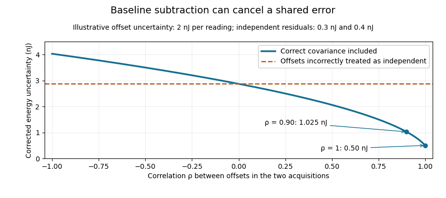
Shared baseline errors cancel according to their correlation
. Original numerical model with a 2 nJ offset uncertainty in each acquisition and independent residual uncertainties of 0.3 nJ and 0.4 nJ. The comparison curve incorrectly treats the shared offsets as independent. Details.A sampled implementation has the same structure. If a vector of readings has covariance matrix , and fixed integration weights give and , thenA constant offset cancels when the weights sum to the same gate duration: . This does not justify using pulse-contaminated readings as background. Matched blank sequences, collected with the actual timing, help characterize the needed noise correlations.
The historical NIST TC-24 apparatus used a thermocouple-based absorbing plate and averaged baseline measurements before and after laser injection to compensate background and thermal drift.[ref]
Calibration Service for Low-level Pulsed-Laser Radiometers at 1.06 µm: Pulse Energy and Peak Power by Rodney W. Leonhardt. §3.5, printed p. 8; §7.2, Leakage Effect
The offset model above is an independent illustration, not a reconstruction of that instrument's uncertainty budget.A differential inequality for an exponential tail envelope supplies a sufficient decay condition for a global power bound. Let nonnegative be absolutely continuous on every finite interval after , with andalmost everywhere, for constant . The integrating factor argument in bounding unobserved optical energy with an exponential tail model gives . Corners in the waveform are allowed under absolute continuity; an unmodeled upward jump is not.
The inequality is stronger than merely fitting a decay constant at a few sampled times. For example, obeys it and carries only after . The exponential-envelope tail-energy bound remains valid but need not be tight. Conversely, a later pulse can violate the differential condition while leaving all earlier samples unchanged.
A useful extension is a time-dependent decay-rate envelope. For locally integrable , the condition givesThis follows from the same integrating factor and is a scalar comparison bound. If throughout the tail, its integrated energy is at most .
For an original piecewise rate, choose , for the first and thereafter. Integrating the resulting continuous envelope yieldsUsing only the minimum rate would give . Faster guaranteed late decay tightens the result.
This is a conditional mathematical proof. A measured electrical waveform obeying a similar slope rule does not establish the optical condition without accounting for the detector impulse response. The primary NIST measurement procedure supplies an example of characterizing that response independently.[ref]
Calibration Service for Low-level Pulsed-Laser Radiometers at 1.06 µm: Pulse Energy and Peak Power by Rodney W. Leonhardt. Appendix C.1–C.2, printed pp. 36–37
The directional derivative of a clipped logarithmic acquisition time describes the first-order recording extension when several envelope parameters change together at the acquisition threshold. For positive , writeThe logarithmic tail-duration change at the zero-extension boundary article treats a fixed decay time and logarithmic input coordinate. Here consider a boundary point and an additive parameter direction .
The one-sided directional derivative uses positive step sizes:The logarithmic chain rule gives the expression inside the maximum. Differentiating the prefactor contributes zero at the boundary because the clipped logarithm there is zero.
For an original example, let , and . Increase amplitude in direction while decreasing decay time in direction , with . The net fractional direction is , so per unit step. Reversing the direction gives derivative zero, not .
The derivative is positively homogeneous in the direction but is not linear, so no single gradient represents all threshold-crossing perturbations. Above threshold the usual smooth derivative applies; strictly below threshold all sufficiently small changes leave the extension zero. Gaussian input uncertainty at a clipped acquisition-time threshold can consequently produce a mass of outcomes exactly at zero rather than a symmetric distribution around a nominal duration. The directional calculation alone does not assign a confidence level.
This is a conditional optical-envelope calculation. Separating optical power from the receiver's electrical response remains necessary before its parameters describe missed light. NIST independently characterized the detector/cable/oscilloscope response in its pulse calibration procedure.[ref]
Calibration Service for Low-level Pulsed-Laser Radiometers at 1.06 µm: Pulse Energy and Peak Power by Rodney W. Leonhardt. Appendix C.1–C.2, printed pp. 36–37
A derivative can describe parameter sensitivity accurately while the envelope itself still needs experimental justification.An empty physical confidence set for a detector variance difference occurs when the entire reported interval for the inferred response variance lies below its admissible range. In the nonnegative-profile detector model, . An interval gives a physical width setIt is empty exactly when . The coverage-preserving detector-width bound from a variance interval proves why this intersection and transformation retain the original coverage event.
For an original reading, suppose an explicitly normal measurement model for gives with known standard deviation . The approximately 95 percent interval contains no nonnegative variance. This is disagreement between that interval and the physical model, not a negative physical detector width or an exact measurement of zero width.
Empty sets can occur occasionally even when the model is correct. If and , thenwhere is the standard normal cumulative distribution function. At the physical boundary and , the probability is about ; at it is about . The boundary probability of an empty detector-width confidence set explains why one empty realization is not a logical disproof of the detector model.
Replacing an empty set by the point zero changes the procedure. It must not be presented as though the original interval precisely determined that point. NIST likewise distinguishes an uncertainty interval from an automatically justified confidence level, emphasizing the distributional assumptions behind coverage factors.[ref]
In practice, examine the width estimates, their correlations and the physical convolution assumptions, while retaining the actual negative interval in the measurement record. NIST's short-input receiver-response measurement illustrates how an independently characterized input helps resolve detector broadening.[ref]
Calibration Service for Low-level Pulsed-Laser Radiometers at 1.06 µm: Pulse Energy and Peak Power by Rodney W. Leonhardt. Appendix C.1–C.2, printed pp. 36–37, Figure C1
Neither clipping the estimate nor declaring the response model false follows solely from the sign of one noisy variance difference. Exponential-envelope tail-energy bound 2026-11-05
An exponential-envelope tail-energy bound limits unobserved energy by integrating a justified pointwise envelope on the true optical power. If for every , with and , then . The parent bounding unobserved optical energy with an exponential tail model derives this result and distinguishes it from a statistical uncertainty.
At a later acquisition endpoint , the remaining allowance isFor an original envelope with and , the initial allowance is . Reducing the allowed missing energy to requires . This acquisition duration from an exponential tail-energy tolerance reduces the bound by a factor100. It does not prove that99% of an arbitrary underlying pulse has been captured: the actual power may lie strictly below the envelope at early times.
Joint parameter constraints also matter. An original allowed set uses dimensionless and with , and . Since , every allowed envelope satisfiesattained at . Taking separate maxima and would instead give the looser bound; those two maxima cannot occur together in the stated joint set.
The guarantee concerns optical power, not an uncorrected detector tail. Optical tail and detector-response ambiguity explains that distinction, while NIST's primary response-calibration procedure characterizes the electrical measurement chain separately.[ref]
Calibration Service for Low-level Pulsed-Laser Radiometers at 1.06 µm: Pulse Energy and Peak Power by Rodney W. Leonhardt. Appendix C.1–C.2, printed pp. 36–37
A delayed extra pulse or an unbounded constant background requires its own model; neither is excluded by a local exponential fit.Finite-input correction in pulse-detector calibration removes the known input duration from an inferred receiver width, while propagating uncertainty in both widths. Under the nonnegative, normalized, finite-variance convolution model of known-input calibration of a pulse detector,where is the known input profile, the measured output and the receiver's impulse response. The subtraction concerns temporal variances, not arbitrary reported full widths.
Differentiating on the positive-width branch givesFirst-order propagation of standard uncertainty therefore yieldsThe covariance matters when both widths use the same timebase or fitted reference.[ref]
An original near-resolution example has and , each with independent standard uncertainty . The corrected receiver width is and its propagated standard uncertainty is about , or . Width measurements individually precise to about one percent can thus give a much less precise difference-derived width.
NIST's primary bandwidth-correction procedure used roughly 120 ps optical inputs and recorded the detector, cable and oscilloscope as one response chain at different gains and signal levels.[ref]
Calibration Service for Low-level Pulsed-Laser Radiometers at 1.06 µm: Pulse Energy and Peak Power by Rodney W. Leonhardt. Appendix C.1–C.2, printed pp. 36–37, Figure C1 and steps 1–7
A sufficiently short characterized input reduces this resolution-limit conditioning in finite-input detector calibration. Near a zero variance difference, linear uncertainty propagation may fail; a nonpositive measured difference does not represent a negative physical detector width. Report an interval or limit under the stated model rather than silently replacing the difference by zero. Negative ringing also violates the nonnegative-profile assumption behind the variance subtraction.Future-domain validity of a fitted power-law optical envelope means that the bound applies throughout the unobserved future interval where its integral is used, rather than merely matching a recorded waveform. The validated lower bound on a power-law tail exponent supplies a sufficient differential condition for such a bound. Agreement on a finite observation window alone does not establish it.
A concrete counterexample uses a fitted profile observed only for . Choose a later time and define an additional pulseBoth and are nonnegative and continuously differentiable, and they agree exactly on the recorded interval. Yet the unobserved extra energy isThus nonnegativity, this degree of smoothness and even a perfect finite-window fit cannot exclude an arbitrarily large later contribution.
For an original example, take , and . The fitted profile predicts remaining energy , below a tolerance. Put the later pulse at with width and peak . It adds , although all recorded data are unchanged. This unobserved delayed-pulse counterexample to a fitted tail bound violates the claimed missed-energy tolerance without altering the fit quality.
To use the envelope as a guarantee, state the physical assumptions that exclude such later input, justify the rate bound over the required future interval, or limit the claim to the interval actually validated. Recording a longer finite window improves evidence but does not alone supply an all-future theorem under only the assumptions used in this counterexample.
The waveform must also represent optical power rather than detector response. NIST's primary pulse calibration separately characterized the detector/cable/oscilloscope chain with a short optical input.[ref]
Calibration Service for Low-level Pulsed-Laser Radiometers at 1.06 µm: Pulse Energy and Peak Power by Rodney W. Leonhardt. Appendix C.1–C.2, printed pp. 36–37, Figure C1 and response-measurement procedure
Correcting the receiver is necessary for interpreting the trace, but it does not rule out the additional source pulse constructed here. The example is a mathematical comparison, not a reported failure of that apparatus. Gaussian gate centring error 2026-11-05
The Gaussian gate centring error is , the time displacement between a gate centre and a Gaussian pulse centre. The Gaussian pulse time-gate energy fraction gives the full displaced-gate formula. Equal positive and negative errors collect equal energy in that symmetric model, so an energy deficit alone does not reveal the direction of the misalignment.
A focused expansion explains sensitivity close to the optimum. Let be the centred energy-normalized pulse profile, let , and define . For the Gaussian standard deviation ,Thus the leading quadratic energy loss from centred Gaussian gate timing error is second order, rather than linear in .
For an original example, take a gate as wide as the power FWHM . Its centred fraction is . An error gives from the full formula; the quadratic approximation gives . For this is a displacement, with gate width and total pulse energy unchanged.
A delay scan of a gated readout can locate the maximum, provided the source and gate widths remain stable. Pulse timing jitter produces a distribution of offsets rather than a single deterministic . Also distinguish a gate on optical power from one on a detector's electrical waveform: NIST measured detector impulse responses and used convolution to assess pulse reproduction.[ref]
Calibration Service for Low-level Pulsed-Laser Radiometers at 1.06 µm: Pulse Energy and Peak Power by Rodney W. Leonhardt. §§6.1–6.2, short-pulse response measurement and numerical convolution
Gaussian pulse energy and peak power 2026-11-05
For an isolated Gaussian pulse, the relation between laser pulse energy and peak power depends on the pulse-width convention. Here is the total incident radiant power, the background is zero, and denotes the power full width at half maximum. Integrating over the entire pulse defines its positive energy .
Pulse energy, peak power and average power resolve different information. Consider a Gaussian pulse withThe chosen pulse duration is the full width at half maximum of radiant power: . It refers to radiant power, rather than the wave amplitude of the electric field. The Gaussian integral gives the relation between Gaussian pulse energy and peak power:The pulse energy shape factor is . It equals for this power profile; a rectangular pulse of duration has . Knowing only a width and an integrated energy therefore requires a pulse-shape assumption before inferring peak power.
An equivalent form makes the normalization transparent. Write the pulse centre as , and let denote the standard deviation of its energy-normalized pulse profile:The ratio is a probability density function in the mathematical sense: it is nonnegative, has units , and integrates to one. Here it weights the pulse's energy over time. Its normal distribution profile has mean and variance . This gives without a separate area estimate.
For a stipulated and , the power full width at half maximum is and the peak power is . Confusing the standard deviation with the full width at half maximum would insert the wrong duration into the conversion.
The Gaussian pulse field-envelope width is a second distinct convention. If a fixed spatial field profile gives for a constant , the wave amplitude envelope obeysConsequently its amplitude full width at half maximum is . Inserting into the formula for a power-width input underestimates the true peak power by a factor . State which measured waveform defines the width.
An electrical photodetector trace can also be broadened by its impulse response. The optical pulse-width inference therefore needs a characterized detector response.[ref]
Gaussian pulse time-gate energy fraction 2026-11-05
The Gaussian pulse time-gate energy fraction is the share of an isolated pulse's laser pulse energy admitted by a finite time window. The result below acts on incident optical radiant power. Let be the power full width at half maximum, and first place the pulse centre and the detection time gate centre at zero.
A detection time gate need not collect the whole pulse. Integrating the same profile only over gives the Gaussian pulse time-gate energy fractionwhere is the error function. A gate as wide as the power full width at half maximum collects only , or 76.10% of the pulse energy. The pulse has nonzero Gaussian tails outside that interval. A real readout's impulse response can extend the required integration window further.
Alignment adds a parameter. Let the pulse centre be , the gate centre be , and write the Gaussian gate centring error as . Put . Integrating the normalized Gaussian pulse profile over the gate givesAt the two error function terms reduce to the centred formula above. With and , the captured fraction drops to . The pulse centre then lies on a gate edge. Merely keeping the gate width fixed does not keep its collected energy fixed.
The gate works best when centred. With the centred energy-normalized pulse profile and , differentiation of givesA Gaussian function is an even function about its centre and decreases with distance from that centre. Thus for , and symmetry gives the opposite sign for . The same argument proves that a centred interval maximizes mass for an even unimodal density; unimodality supplies the required monotonicity.
A centred gate of width captures of the energy. Solving gives for 99% capture in this ideal model. The requirement changes if the centring error is nonzero.
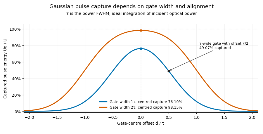


Pulse timing jitter can therefore create variation in gated energy even when every full pulse has the same . A wider gate reduces this loss but also changes admitted background and the chance of including neighbouring pulses. Measure the timing and detector response associated with the chosen gate.
For a detector modeled as a linear time-invariant system, its recorded waveform is a convolution of the optical input with its impulse response. NIST tested avalanche photodiode radiometers with roughly optical pulses, recorded their responses with an oscilloscope, and convolved measured responses with longer Gaussian inputs to estimate corrections. The detector and amplifier were characterized together.[ref]
Calibration Service for Low-level Pulsed-Laser Radiometers at 1.06 µm: Pulse Energy and Peak Power by Rodney W. Leonhardt. §§6.1–6.2, printed pp. 13–15: short-pulse excitation, sampling readout and numerical convolution
A gate applied to that electrical waveform must use the readout model rather than assuming the optical fraction is unchanged.