
Radiant exposure 2026-11-05
Radiant exposure measures the radiant energy received per unit surface area during a specified interval. At a fixed surface point , it is the time integral of incident irradiance :The area belongs to the receiving surface: its orientation and location matter. An irradiance in specifies a rate, while radiant exposure in specifies the accumulated arrival of energy.[ref]
International Lighting Vocabulary by CIE. CIE S 017:2020, entry 17-21-071, definition, symbols and note 3
For a uniform rectangular pulse, , with constant irradiance and duration . Stipulate one pulse at for , and another at for . Both deliver , but their peak irradiances differ by a factor of four. The two radiant exposures agree only after each complete pulse has arrived. A shorter observation window can intercept different fractions of them, and a nonlinear receiver can respond differently even to their complete pulses.
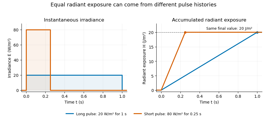
Original rectangular-pulse example: different irradiance histories accumulate the same radiant exposure.
Details. 
Integrating over a receiving patch gives its incident radiant energy:Here is the spatially averaged radiant exposure, rather than necessarily the local maximum. Uniform illumination is the special case where this spatially averaged radiant exposure equals the local value everywhere on the patch. In the rectangular-pulse example, a uniformly illuminated patch receives .
For an original spatial example, consider a circular Gaussian beam at a fixed transverse plane, with constant Gaussian beam radius throughout the pulse. Let be its total radiant power and its laser pulse energy. Integrating its transverse irradiance in time gives the radiant exposure of a Gaussian beam:The normalization follows by integrating from to . The disk of radius contains only , so its actual spatially averaged radiant exposure is , not . With stipulated and , the peak is , while the average inside that disk is . State the Gaussian beam radius convention and the receiving area with any reported value.
An energy readout alone therefore does not specify a surface's radiant exposure. In an ideal linear model for pulse energy measurement with a photodiode, dark-subtracted photocurrent has constant spectral responsivity at the chosen wavelength. Integrating the electric current gives signal electric charge . If a known patch of area is uniformly illuminated and all of its incident energy is collected, thenAs a separate stipulated example, and correspond to . Uniform illumination over gives . Background subtraction, collection geometry, detector linearity and an integration window covering the full response are part of this measurement model. Continuous-wave responsivity alone does not establish linearity for a short pulse: silicon-photodiode experiments have observed pulse-dependent saturation.[ref]
Measuring Pulse Energy With Solid-State Photodiodes by Robert E. Vest and others. Abstract: pulsed nonlinearity and dependence on reverse bias and illuminated area
A historical NIST measurement calibration separates these operations experimentally. A modulator produces pulses from a continuous-wave laser; a calibrated beam splitter sends one beam to a slow thermal reference and another to the pulse detector. The reference records the accumulated energy, while the pulse repetition rate and injection duration determine the mean energy per pulse. The detector's integrating electronics provide a pulse-energy readout. Converting such a readout to radiant exposure additionally requires the illuminated area and its spatial distribution.[ref]
The beam-use term fluence denotes the same time integral for a directed beam normal to the chosen surface. For light arriving from many directions, specify the angular geometry: planar irradiance and spherical irradiance are different quantities, so a value defined using one cannot simply be substituted for the other.[ref]
International Lighting Vocabulary by CIE. Entry 17-21-054, notes 1–2: directional radiance and the small-sphere construction
Receiver-latency uncertainty in the inferred input-time horizon propagates uncertainty in timing calibration into the latest input time that could have influenced a stored output record. For one channel, the horizon in input-time horizon of a delayed optical receiver record is , with last output time and effective input-to-output timing offset . HenceThis linear variance identity retains shared timing influences.[ref]
A common calibration offset can cancel when it enters both quantities. In an original model, let errors be and , with independent components of standard deviations , and . Then and . Discarding their common-offset covariance would instead give .
The shared component must come from the actual calibration model. Here is the effective timing offset relating the input and output coordinates, so an output-clock alignment error can enter both and . A physical transport-delay error is not automatically correlated with the last-sample timestamp.
For hard timing limits, propagate validated bounds rather than reinterpret standard uncertainty as a guarantee. If is known and , then . Claiming the optimistic endpoint as though it held for every allowed delay would overstate the input-time reach.
With several channels, . Channel switching under uncertainty in a combined receiver horizon makes this a nonsmooth function when the maximizing channel is uncertain. Propagate the justified joint timing set or distribution; a derivative of only one nominally best channel can miss such switching.
NIST's primary pulse calibration measured the detector, cable and oscilloscope together using a short known optical input.[ref]
Calibration Service for Low-level Pulsed-Laser Radiometers at 1.06 µm: Pulse Energy and Peak Power by Rodney W. Leonhardt. Appendix C.1–C.2, printed pp. 36–37, Figure C1
The numerical timing errors above are chosen examples, not values from that apparatus. A timing horizon remains a necessary information limit; it does not guarantee invertibility of the receiver or bound future optical illumination.Resolution-limit conditioning in finite-input detector calibration is the sensitivity of a small inferred detector width to uncertainty in two nearly equal measured widths. In finite-input correction in pulse-detector calibration, the nonnegative normalized convolution model givesThe signed relative sensitivities areThey diverge as the measured output width approaches the known input width . Subtracting two well-measured squared widths can therefore be a poorly conditioned inference.
For an original example, and give and . The two relative sensitivity coefficients are about and . A small independent fractional width error can produce a much larger fractional response-width error; a common multiplicative timebase error instead partly cancels because the coefficients sum to one. Correlations must therefore be retained.[ref]
Near the boundary, report uncertainty in the variance difference before transforming it. For a chosen interval , imposing the physical constraint gives a detector-width interval , approximately . A coverage-preserving detector-width bound from a variance interval uses this monotone square-root transformation on the physical intersection. It need not resemble a symmetric error bar around a point estimate. An interval wholly below zero contains no admissible width under this model; replacing it silently with a zero-width result hides the inconsistency.
NIST characterized its detector/cable/oscilloscope chain with an optical pulse much shorter than the receiver response.[ref]
Calibration Service for Low-level Pulsed-Laser Radiometers at 1.06 µm: Pulse Energy and Peak Power by Rodney W. Leonhardt. Appendix C.1–C.2, printed pp. 36–37; approximately 120 ps optical input and Figure C1
That design avoids subtracting two nearly equal broad widths. The variance identity still requires nonnegative profiles and finite second moments; arbitrary full widths at half maximum and responses with negative ringing need a different model.A response-normalized tolerance for baseline-feasibility residuals measures a pulse estimator's constraint errors against physically chosen response limits. For residual , assign positive tolerances in the corresponding response units and calculateThe criterion means every specified response limit is satisfied. Numerical feasibility residual for baseline constraints explains why a raw unscaled norm alone has no universal physical interpretation.
These tolerances can enforce a deterministic bias budget. If signal and background coefficients are bounded by and , thenThe second inequality follows when the normalized test passes. The allocation of a deterministic bias budget among baseline constraints therefore connects a numerical acceptance criterion to a stated physical error allowance.
For an original example, bound the signal amplitude by , constant background by and drift rate by . Choose signal-response tolerance , constant-response tolerance and linear-time-response tolerance . Their maximum bias contributions are respectively , and , totaling . If all actual residuals are half these tolerances, and the corresponding bias bound is .
The normalized test can be invariant to constraint units. Multiplying one equation and its required response by a nonzero factor multiplies its residual by ; replacing its tolerance by keeps the ratio unchanged. The associated coefficient bound changes inversely, so the physical product is unchanged as well.
NIST's before/after pulse baselines supply a measurement setting where residual offset and drift responses matter.[ref]
Calibration Service for Low-level Pulsed-Laser Radiometers at 1.06 µm: Pulse Energy and Peak Power by Rodney W. Leonhardt. §3.5, printed p. 8; §7.2, Leakage Effect
The example bounds and tolerances are stipulated, not specifications of that apparatus. This deterministic leakage test is separate from noise variance, which needs the actual measurement covariance.[ref]Guidelines for Evaluating and Expressing the Uncertainty of NIST Measurement Results by Barry N. Taylor and Chris E. Kuyatt. Appendix A, equation A-3
Backgrounds outside the assumed family also need separate treatment. Rodney W. Leonhardt 2026-11-05
Rodney W. Leonhardt is the author of a2004 National Institute of Standards and Technology report on measurement calibration of low-level pulsed-laser radiometers at a wavelength of1.06micrometres. It treats laser pulse energy and peak power as separate measurement quantities and describes the apparatus and measurement uncertainty needed to transfer a laboratory reference to a test instrument.[ref]
Calibration Service for Low-level Pulsed-Laser Radiometers at 1.06 µm: Pulse Energy and Peak Power by Rodney W. Leonhardt. NIST SP250-64, title/byline and §§3–5
The pulse-energy procedure uses a modulated laser, a calibrated beam splitter arrangement, a relatively slow thermal reference and a fast test radiometer. The reference accumulates energy over many pulses. Pulse repetition rate and the illumination interval determine the pulse count; the splitter ratio transfers the reference energy to the lower-energy test beam. The thermal detector need not resolve individual pulses.[ref]
For an original idealized transfer calculation, let the reference receive a total over equal pulses. Define as the reference-to-test beam energy ratio. The average energy per test pulse isIf the calibrated radiometer's selected output measure is0.20volts, the corresponding energy-per-output coefficient would be50picojoules per volt. These invented values explain the transfer arithmetic and do not reproduce the report's calibration results.
The output measure must be specified together with its coefficient. Leonhardt's report discusses offsets in the integrating-amplifier waveform and use of peak-to-peak electric potential difference as a readout. Its peak-power procedure separately compares continuous and pulsed conditions.[ref]
Calibration Service for Low-level Pulsed-Laser Radiometers at 1.06 µm: Pulse Energy and Peak Power by Rodney W. Leonhardt. §4, waveform/offset discussion; §5.1, peak-power comparison
The work illustrates how a measurement becomes reproducible by recording the optical transfer and electrical readout conventions, rather than only stating a detector sensitivity.Simpson baseline integration for pulse-energy correction subtracts a three-point estimate of integrated background from a measured gate integral. For a baseline on , Simpson's rule givesIt is exact for a quadratic or cubic baseline, provided the three values represent background rather than pulse-contaminated samples. For a four-times differentiable baseline, the remainder is for some .[ref]
3.5 Quadrature, subsection (ii) Simpson’s Rule. equation3.5.6, elementary rule and fourth-derivative remainder
For an original chosen quadratic background, take with beginning, midpoint and end values , and . Its integrated baseline is , whereas endpoint averaging would give . A raw gate integral of therefore gives after the three-point correction. Overestimating only the midpoint by would subtract an extra .
The uncertainty of a three-point baseline integral is separate from its quadrature error. With baseline-sample covariance matrix and , its variance is . Independent samples of common standard uncertainty give ; a perfectly shared additive baseline error of the same uncertainty gives instead. Covariance terms cannot be discarded.[ref]
A matched blank acquisition or independently measured background can supply the midpoint. Historical NIST pulse-energy apparatus used before/after baselines for background and thermal-drift compensation.[ref]
Calibration Service for Low-level Pulsed-Laser Radiometers at 1.06 µm: Pulse Energy and Peak Power by Rodney W. Leonhardt. §3.5, reference-standard processing; §7.2, Leakage Effect
The three-point example is an original extension, not a claim about that instrument's processing. Higher polynomial exactness does not compensate for an incorrectly identified baseline. Temporal energy centroid of an optical pulse 2026-11-05
The temporal energy centroid of an optical pulse is its energy-weighted mean time. For nonnegative radiant power with finite positive energy and finite absolute first moment,The normalization uses radiant energy as integrated radiant flux.[ref]
International Lighting Vocabulary by CIE. entry 17-21-041, note 1
The centroid is a moment of the energy-normalized pulse profile; it need not coincide with the largest power value, a threshold crossing or the middle of the FWHM interval.For an original two-component example, let ninety percent of the energy belong to a symmetric narrow component centred at zero and ten percent to a symmetric component centred at . Linearity of the integral gives . Weak delayed energy can move the centroid even when the dominant peak remains near zero. Multiplying the whole power trace by a positive constant leaves unchanged; translating it by shifts its centroid by .
A detector response can shift the measured centroid too. Suppose a normalized impulse response and normalized optical profile have finite absolute first moments. For their convolution , direct integration with givesThus a causal exponential detector response of time constant shifts the recorded centroid by in this model. NIST's pulsed-radiometer characterization explicitly measures detector impulse responses and uses convolution to assess reproduced waveforms.[ref]
Calibration Service for Low-level Pulsed-Laser Radiometers at 1.06 µm: Pulse Energy and Peak Power by Rodney W. Leonhardt. §§6.1–6.2, printed pp. 13–15
The centroid identity is the independent moment calculation above.Baseline drift can cause a separate shift. Suppose a true pulse has and , but a positive residual baseline of remains across the analysis window from to . Its added energy is , centred at . The resulting centroid isA waveform measurement should therefore record the time window, baseline estimate and detector timing response with its reported centroid. A negative background-subtracted trace also needs care: it is not automatically a nonnegative energy distribution.
Thresholded stopping of a capped-tolerance multiplier search ends a numerical allocation when a feasible physical budget is sufficiently well used. With the decreasing budget function in tolerance-budget residual bound for multiplier bisection, an exact upper bracket endpoint satisfies . A residual requirement is , where has the same physical units as the permitted deterministic bias . A small change in alone does not establish that condition.
Numerical evaluation also needs a bound. Suppose the reported value has validated absolute error . Both feasibility and the residual requirement are certified ifEquivalently, the acceptable reported value lies inThis window is empty if . Iterating the multiplier more accurately cannot by itself overcome an evaluation-error bound larger than the desired physical certificate.
For an original numerical certificate, let , and . Values are certifiable. A reported places the actual budget in , so it is feasible and leaves at most unused. A reported is closer to ten but could represent and therefore does not certify feasibility.
The evaluation allowance must itself be justified, for example by validated arithmetic or an explicit forward-error analysis. Uncertain physical coefficients also need their stipulated worst-case bounds before the numerical sum can certify the physical error. NIST's pulse-radiometer discussion motivates the offset and leakage terms; it does not provide the hypothetical numerical tolerances above.[ref]
Calibration Service for Low-level Pulsed-Laser Radiometers at 1.06 µm: Pulse Energy and Peak Power by Rodney W. Leonhardt. §3.5, printed p. 8; §7.2, Leakage Effect
Time-dependent decay-rate envelope 2026-11-05
A time-dependent decay-rate envelope bounds a nonnegative signal using a lower bound on its instantaneous decay rate. If is absolutely continuous on finite intervals, and almost everywhere for locally integrable , thenThe differential inequality for an exponential tail envelope article proves this comparison using an integrating factor and gives a piecewise-constant example. A strictly positive constant lower bound on gives exponential decay, but a positive rate at every instant need not supply such a lower bound.
An original example takes with and . Its integrated rate is logarithmic, soThis power-law tail from a decaying rate envelope tends to zero for every positive . Its envelope energy is nevertheless finite only when , in which caseFor original chosen , and , the allowance is . After a further it is at most . The remaining energy decreases algebraically rather than exponentially.
At the integrated envelope diverges logarithmically despite its power tending to zero. This does not prove that every signal below it has infinite energy; it means these assumptions alone supply no finite all-time energy bound. Taking the envelope itself gives a mathematical counterexample to the claim that pointwise decay implies integrable energy.
An experimental rate law therefore needs both temporal validity and an integrability check before it bounds missed optical energy. A measured detector tail is not automatically the true power profile; NIST's primary calibration procedure measures the receiver response separately.[ref]
Calibration Service for Low-level Pulsed-Laser Radiometers at 1.06 µm: Pulse Energy and Peak Power by Rodney W. Leonhardt. Appendix C.1–C.2, printed pp. 36–37
The power-law example is an independent comparison model, not a reported tail law of that apparatus.A tolerance-budget residual bound for multiplier bisection controls the physical bias left unused by a numerical allocation, rather than only the numerical error in its Lagrange multiplier. Use from monotonicity of the multiplier equation for capped tolerances. Suppose a positive bracket satisfies . Choosing the upper endpoint gives a feasible allocation, with residualChoosing the lower endpoint can violate the budget. The direction of monotonicity therefore matters even when both endpoints are numerically close.
For an a priori bound, put . On the entire bracket, each summand obeys Lipschitz continuity with constant at most , including across its breakpoint. HenceAfter bisections of an original bracket with , the corresponding worst-case bound is . This is conservative; evaluating the two endpoint budgets can give a much tighter residual certificate.
For an original stopping example, use , and in common normalized bias units. The bracket straddles the root. Its feasible upper endpoint leaves unused. One bisection evaluates and replaces the upper endpoint, reducing that unused amount to about . A residual allowance of is now met, despite a breakpoint lying inside the bracket.
This gives a thresholded stopping of a capped-tolerance multiplier search in the same units as the permitted bias. Floating-point comparisons also need an allowance for rounding if they are to serve as hard certificates. The underlying bias coefficients and cost model remain assumptions of cost-weighted allocation of baseline-response tolerances; numerical precision cannot validate missing physical terms. NIST's pulse-radiometer account motivates the offset/leakage constraints rather than prescribing this numerical stopping rule.[ref]
Calibration Service for Low-level Pulsed-Laser Radiometers at 1.06 µm: Pulse Energy and Peak Power by Rodney W. Leonhardt. §3.5, printed p. 8; §7.2, Leakage Effect
A two-channel covariance estimate of pulse-energy variance uses the component shared by paired readouts to estimate source fluctuations. In a stipulated linear model let and , with calibrated nonzero gains. If both noise terms are uncorrelated with and with each other,This follows by expanding the covariance. Correlation assumptions are essential measurement-model inputs; the uncertainty guide retains covariance terms explicitly.[ref]
For an original example, choose , and measured covariance . The inferred source variance is , giving a standard deviation of . Independent readout-noise variances and would give total variances and while preserving that cross-covariance.
But a shared noise covariance of raises the observed cross-covariance to . Ignoring it would infer a source standard deviation of , about too high.
A split-beam experiment records both channels for the same pulses, checks gains and measures dark or independent-input controls for correlated electronics. NIST's calibrated splitting apparatus supplies an example of the optical geometry, not a claim that it used this covariance estimator.[ref]
Calibration Service for Low-level Pulsed-Laser Radiometers at 1.06 µm: Pulse Energy and Peak Power by Rodney W. Leonhardt. §3.4, calibrated beam splitting
Matching pulse indices, bandwidth and integration windows is part of the proposed model.An unobserved delayed-pulse counterexample to a fitted tail bound constructs two admissible optical inputs giving the same finite measurement record but different missed energies. The future-domain validity of a fitted power-law optical envelope article gives a nonnegative, continuously differentiable delayed pulse with adjustable energy. The counterexample persists through a calibrated causal detector, not just an ideal instantaneous power readout.
Let , where the additional pulse has support after the record ends at . A linear receiver with impulse response and responsivity measures . Causality means for . Therefore, for every recorded time ,since every argument is negative. This causal indistinguishability of delayed optical inputs on a finite record holds even when the impulse response is known exactly and the recorded data are noiseless.
For an original example, record through and place the smooth sine-squared pulse of the parent article at , with width and peak . Its extra optical energy is . A chosen causal exponential receiver with decay time produces no difference in the initial record, although it will respond when the later pulse arrives. If its impulse response has unit area, the complete later output-area difference is in the receiver's output-area units.
Any rule using only the common initial record must return the same proposed bound for both inputs. Without a justified restriction on later illumination, the delayed pulse energy can be chosen larger than any proposed finite guarantee. More accurate calibration of that same initial record cannot resolve this information gap.
NIST characterized its detector, cable and oscilloscope together with a short known optical input before correcting pulse measurements.[ref]
Calibration Service for Low-level Pulsed-Laser Radiometers at 1.06 µm: Pulse Energy and Peak Power by Rodney W. Leonhardt. Appendix C.1–C.2, printed pp. 36–37, Figure C1 and response-measurement procedure
Such response calibration addresses receiver distortion. Source shutoff, exclusion of later pulses or a future-valid rate envelope supplies the additional physical information needed for a missed-energy guarantee. The delayed pulse here is a mathematical construction, not a reported defect of that apparatus.A validated lower bound on a power-law tail exponent is an exponent constraint that is justified over the future interval where it is used to bound unrecorded energy. A fitted slope over a finite observation window is not by itself such a guarantee. Acquisition duration from a power-law tail-energy tolerance needs a global optical-power envelope, including a lower exponent limit above one for its finite-energy guarantee.
One sufficient condition, for positive absolutely continuous power, isIntegrating the logarithmic derivative gives . The time-dependent decay-rate envelope provides the equivalent integrating-factor argument when zeros of the power need handling. This is a sufficient condition, not a necessary characterization of every bounded tail.
For an original conditional estimation example, assume an exact power-law family with known and initial power . At , a measured ratio range yieldsapproximately . Within that assumed family, the lower endpoint gives a conservative extension about for a remaining-energy tolerance. A nominal exponent two would instead require .
The ratio interval constrains the exponent only conditional on the exact family, known time scale and suitable measurement uncertainty. It cannot exclude a later secondary pulse or a transition to a slower law after the observed window. Future-domain validity of a fitted power-law optical envelope therefore requires independent physical justification or explicitly limited claims. If the justified exponent set reaches one, this envelope alone supplies no finite all-time energy guarantee.
Finally, the measured trace must represent optical power rather than an uncorrected receiver tail. NIST measured the detector, cable and oscilloscope together using a short characterized optical input before correcting pulse measurements.[ref]
Calibration Service for Low-level Pulsed-Laser Radiometers at 1.06 µm: Pulse Energy and Peak Power by Rodney W. Leonhardt. Appendix C.1–C.2, printed pp. 36–37, Figure C1 and response-measurement procedure
The exponent example is an original model calculation, not an observed law attributed to that apparatus.