
The input-time horizon of a delayed optical receiver record is the latest physical input time that could influence the recorded output, given the receiver's causal onset delay. If for and the last output time is , convolution depends only on input timesThus is a necessary timing limit on information in that record. Recoverability within the limit additionally depends on bandwidth, noise, sampling and the response's invertibility. Causal indistinguishability of delayed optical inputs on a finite record shows why later input changes cannot be inferred from the existing output samples.
For several channels with last recorded times and known onset delays , the latest possible input horizon isAny input perturbation starting strictly after is invisible in every stored channel. A channel's latest output timestamp alone is insufficient to compare its input horizon with another channel's.
For an original example, channel 1 records through with delay , while channel 2 records through with delay . Their input limits are and ; the combined limit is . Knowing both response functions exactly still supplies no observation of an input pulse beginning later than that limit.
A receiver-latency uncertainty in the inferred input-time horizon also changes the timing claim. If channel 1's delay is known only to lie between and , its possible horizon ranges from to . An input beginning at could affect the record for one allowed delay but arrive too late for another. Using the conservative endpoint avoids claiming timing access that depends on an unresolved latency. It still does not guarantee successful reconstruction of every earlier input.
NIST characterized detector, cable and oscilloscope as a combined response chain using a short known optical pulse.[ref]
Calibration Service for Low-level Pulsed-Laser Radiometers at 1.06 µm: Pulse Energy and Peak Power by Rodney W. Leonhardt. Appendix C.1–C.2, printed pp. 36–37, Figure C1 and response-measurement procedure
Such a calibration must relate output timing to the physical input time origin. The delays above are illustrative, not quoted apparatus values. De-embedding known latency aligns the record's time reference; it cannot extend observations into an unrecorded future interval. Known-input calibration of a pulse detector 2026-11-05
Known-input calibration of a pulse detector uses a characterized optical waveform to separate the incident signal from the receiver response. In a linear, baseline-corrected model,where is known input power, a normalized impulse response and the overall responsivity. Recording the complete response givesThus a known reference energy calibrates the area gain without requiring the input to be an ideal impulse. Shape calibration additionally uses the reference waveform.
For nonnegative normalized profiles with finite second moments, define and . Since , their temporal variances satisfy . In an original chosen example, an input standard deviation and recorded deviation imply . Treating that finite input as a delta impulse would incorrectly assign the full to the detector. This finite-input correction in pulse-detector calibration concerns standard deviations; a universal subtraction rule for arbitrary FWHM values does not follow. Negative ringing also invalidates the nonnegative-profile interpretation used for the variance identity.
NIST's primary procedure illuminated the detector with a pulse much shorter than the detector response and characterized detector, cable and oscilloscope together at the relevant gain and signal levels.[ref]
Calibration Service for Low-level Pulsed-Laser Radiometers at 1.06 µm: Pulse Energy and Peak Power by Rodney W. Leonhardt. §§6.1–6.2; Appendix C.1–C.2, printed pp. 36–37, Figure C1 and measurement procedure
Such a known input breaks the optical tail and detector-response ambiguity described by the parent article.In the frequency domain, the same model is . Division can estimate where the input spectrum is known and sufficiently nonzero; small input components amplify measurement noise. A short reference pulse is useful because it excites a broad frequency range, but detector linearity, baseline, area coverage and reference uncertainty still need checking.
Laser pulse energy 2026-11-05
Laser pulse energy is the radiant energy carried by one specified laser pulse across a measurement plane. For an isolated pulse whose total radiant power is and whose background is zero,Here is already integrated over the transverse beam area; it is not local irradiance. The unit of is the joule. Radiant exposure instead divides received energy by a receiving area, so a beam's alone does not specify the exposure at its centre. The radiant exposure of a Gaussian beam makes that spatial distinction quantitative.
The Gaussian pulse energy and peak power relation gives when is the power full width at half maximum. The pulse energy shape factor records pulse-shape dependence, while the Gaussian pulse field-envelope width is times the power width.
For an original example, stipulate and a Gaussian pulse power full width at half maximum . Then . Stretching the same model pulse to while keeping unchanged reduces its peak power to . Both curves below integrate to the same energy; their peak heights and widths differ.
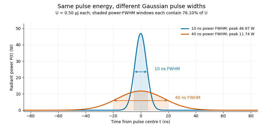

A finite detection time gate collects the Gaussian pulse time-gate energy fraction, which depends on its width and alignment. A centred gate as wide as the power full width at half maximum receives only of , because Gaussian tails extend beyond it. For a -wide gate, a Gaussian gate centring error of reduces capture to .
The average power of a laser pulse train follows by counting complete pulses. If a long observation of duration contains pulses of energies , with negligible edge contributions and no continuous background,Here is the pulse repetition frequency, not the inverse pulse width. An average power readout constrains when is known; it does not resolve pulse-to-pulse energy fluctuation. Identical, well-separated pulses at give average power, even though the stipulated pulses peak near .
If a steady optical background is present, state whether the reported energy includes it. For pulse energy above a measured background , the pulse energy baseline correction uses . Failing to subtract a constant background adds to the inferred energy. This optical-background model is distinct from an offset introduced later by detector electronics.
Historical NIST equipment illustrates what the readouts measure. Its TC-24 reference absorbed the beam in a glass plate, sensed a plate temperature difference with thermocouples, and integrated the thermopile's electric potential difference during beam injection. Before/after readings enabled background subtraction and compensated thermal drift. Counting pulses converted total injected energy to mean pulse energy. The semiconductor pulse photodetector used an integrating amplifier; calibration related the peak output electric potential difference to pulse energy. That electrical peak did not by itself establish optical peak power.[ref]
Calibration Service for Low-level Pulsed-Laser Radiometers at 1.06 µm: Pulse Energy and Peak Power by Rodney W. Leonhardt. §3.5, printed p. 8; §4, printed pp. 9–10: thermal reference, baselines, pulse counting and integrated readout
Pulse energy measurement with a photodiode connects this kind of measurement to collected electric charge; validating the detector response under the actual pulse conditions remains part of that interpretation.Logarithmic condition numbers of a tail-acquisition requirement quantify the fractional response of a positive recording extension to fractional parameter changes. For with , define the signed sensitivity . ThenTheir absolute values are componentwise relative condition numbers. Acquisition-time sensitivity to tail-model parameters gives the corresponding dimensional derivatives and uncertainty propagation.
These numbers depend on which coordinates are held fixed. If denotes the initial tail-energy allowance, then . In coordinates , the decay-time sensitivity at fixed is exactly one, rather than . This is the same physical formula: holding fixed while changing also changes . Transforming the parameter covariance consistently leaves the propagated output uncertainty unchanged.[ref]
An original boundary example takes and . The required extension is only , but . Increasing by multiplies the ratio by , giving and doubling the required extension exactly. Its relative change is large because the original extension was very small.
This does not mean the absolute requirement is singular there. In the active branch remains finite. At and below the threshold, the physical extension is zero, so is undefined. A logarithmic tail-duration change at the zero-extension boundary must instead use the piecewise requirement or absolute changes. Large relative conditioning alone is not evidence of a large absolute recording-time risk.
Finally, conditioning describes the stated envelope model, not its experimental validity. The optical power tail must be distinguished from detector response, which NIST measured independently in its pulse calibration procedure.[ref]
Calibration Service for Low-level Pulsed-Laser Radiometers at 1.06 µm: Pulse Energy and Peak Power by Rodney W. Leonhardt. Appendix C.1–C.2, printed pp. 36–37
A well-conditioned calculation based on an invalid optical envelope still gives an unjustified acquisition guarantee.Logarithmic tail-duration change at the zero-extension boundary describes a recording requirement whose input ratio crosses the point where no further acquisition is needed. For fixed decay time , put and . The physical extension isHere the logarithm applies to the input ratio, not to a zero output duration. Logarithmic condition numbers of a tail-acquisition requirement applies only where .
At , the left derivative is zero and the right derivative is . The directional derivative of a clipped logarithmic acquisition time along a signed input change isThus no single ordinary derivative describes threshold-crossing perturbations. Nevertheless, the duration is stable in absolute units:This follows because the positive-part map has Lipschitz continuity with constant one.
For an original interval example, take and a justified input-ratio range . The corresponding duration range is . Its lower part is clipped at zero. Linearizing only on the zero-duration side would incorrectly predict no possible extension even though the allowed set crosses the threshold. A relative error divided by a nominal is undefined, while this absolute bound remains meaningful.
If is uncertain too, optimize the full expression over the justified joint parameter set rather than treating this fixed- inequality as a complete uncertainty analysis. The tail model must bound optical power throughout the missed interval. NIST's calibration apparatus measured detector/cable/oscilloscope response separately, illustrating why a recorded electrical decay cannot automatically certify such an optical envelope.[ref]
Calibration Service for Low-level Pulsed-Laser Radiometers at 1.06 µm: Pulse Energy and Peak Power by Rodney W. Leonhardt. Appendix C.1–C.2, printed pp. 36–37
The clipping analysis is an original property of the stated conditional acquisition model.Minimum-noise weights under baseline moment constraints choose a linear pulse estimator with the smallest variance among those that preserve a specified signal and remove specified backgrounds. Write the reading vector as , where is a known signal template, the columns of contain baseline shapes, and the error covariance matrix is positive definite. For , requireColumns in implement the moment conditions for baseline-drift cancellation. The noise cost of polynomial baseline cancellation depends on which feasible weights are chosen.
If the constraint columns are independent, Lagrange multipliers giveFor any feasible perturbation , and , so the variance increases by . This proves the minimum and connects the estimator to generalized least squares. The covariance propagation is the full quadratic form, not a sum that discards correlations.[ref]
For an original one-bin pulse example, use five equally spaced times , a signal present only at the centre, and independent errors of variance . To remove just constant and linear backgrounds, the optimal dimensionless weights are . Their variance is , lower than for the centre and its two nearest references alone. Multiplying the amplitude estimate by a bin duration gives energy variance . Extra uncontaminated references can reduce noise when the cancelled background family stays the same.
The inverse requires genuinely independent constraints. Constraint redundancy in baseline-noise minimization calls for removing redundant columns and checking feasibility; a signal template inside the nuisance span cannot be preserved while that span is rejected. NIST's before/after pulse baselines provide the physical measurement context.[ref]
Calibration Service for Low-level Pulsed-Laser Radiometers at 1.06 µm: Pulse Energy and Peak Power by Rodney W. Leonhardt. §3.5, printed p. 8; §7.2, Leakage Effect
The five-point design is an original idealization and assumes no pulse signal in its reference samples.Moment conditions for baseline-drift cancellation specify which polynomial backgrounds a linear measurement removes. Let readings at known times enter the corrected pulse estimate as , with the integration/calibration units included in . A background contributes nothing wheneverSubstitution gives this result directly. The zeroth condition removes a common offset; the first additionally removes linear drift. These conditions concern the actual weights and times, not only the number of background samples.
An original one-bin signal model measures a pulse at , with uncontaminated reference samples at and . UseThe weights sum to zero and have zero first time moment. Constant and linear backgrounds cancel exactly, but a quadratic background leaves bias . With chosen , and , the bias is . Here the pulse is stipulated to occupy the central bin; the formula is not a universal integral estimator for an arbitrary waveform.
Cancellation has a noise cost of polynomial baseline cancellation. For independent equal-variance reading errors , the chosen estimate has variance , even though its constant and linear bias terms vanish. General correlations use instead.[ref]
NIST's historical pulse-energy apparatus used before/after baselines for background and thermal-drift compensation.[ref]
Calibration Service for Low-level Pulsed-Laser Radiometers at 1.06 µm: Pulse Energy and Peak Power by Rodney W. Leonhardt. §3.5, printed p. 8; §7.2, Leakage Effect
The polynomial test above is an original general analysis. Pulse contamination in a reference, uncertain timing or drift outside the assumed polynomial family can leave a residual even when the nominal algebraic conditions hold.Monotonicity of the multiplier equation for capped tolerances makes the allocation in active-set clipping in cost-weighted baseline-tolerance allocation computable by a scalar search, even at a change of active constraints. Express each capped physical bias contribution as . The total allocated bias at positive Lagrange multiplier isEach summand is continuous and nonincreasing. Its breakpoint is ; below that value it is capped, and above it it is strictly decreasing. Between breakpoints,Thus is initially constant at and becomes strictly decreasing once the first component is free. Continuity persists when the derivative changes.
For a binding budget , there is exactly one solution of . It lies in the explicit positive bracketbecause and . The bisection method preserves a bracket without requiring a derivative at the root. A tolerance-budget residual bound for multiplier bisection can then relate the stopping rule to the physical bias budget instead of only to the multiplier's units.
For an original dimensionless illustration, take , , and , with bias expressed in one common reference unit. The bracket is . At , the contributions are and sum to three. This root is itself a breakpoint: the first contribution changes between capped and free there. The derivative is just below it and just above it, while the function remains continuous and strictly decreasing.
The argument uses the positive coefficients and logarithmic effort model specified by the parent. NIST's pulse-radiometer discussion motivates controlling offset and leakage, but does not prescribe that mathematical cost model.[ref]
Calibration Service for Low-level Pulsed-Laser Radiometers at 1.06 µm: Pulse Energy and Peak Power by Rodney W. Leonhardt. §3.5, printed p. 8; §7.2, Leakage Effect
The noise cost of polynomial baseline cancellation is the change in random measurement uncertainty when extra background trends are removed. For a linear pulse estimate and reading-error covariance matrix ,The moment conditions for baseline-drift cancellation constrain to reject specified polynomial backgrounds. They do not make the remaining random error vanish.[ref]
For an original comparison, assume a pulse occupies only the central sample and the other samples contain background alone. Three samples at with weights cancel constant and linear backgrounds. Five samples at can instead useThese weights preserve the central signal and have zero moments of orders . For independent reading errors of equal variance , the three-sample variance is , while the five-sample variance isWith and , the standard uncertainties are approximately and . The second design removes quadratic and cubic drift as well, but its larger reference weights increase noise. This compares two specified estimators; it is not a claim that collecting more background data must worsen precision.
NIST's pulse-energy apparatus used before/after baseline measurements for background and thermal-drift correction.[ref]
Calibration Service for Low-level Pulsed-Laser Radiometers at 1.06 µm: Pulse Energy and Peak Power by Rodney W. Leonhardt. §3.5, printed p. 8; §7.2, Leakage Effect
The polynomial comparison above is an original model for choosing such measurements. Choosing minimum-noise weights under baseline moment constraints can exploit additional reference samples and their measured correlations. Pulse leakage into a reference or drift outside the cancelled polynomial family still creates bias.The null-space feasibility test for baseline-estimator constraints determines whether any measurement weights can preserve a specified pulse response while removing the requested backgrounds. Write the conditions as . The criterion in constraint redundancy in baseline-noise minimization is that be orthogonal to every vector in the kernel of .
A singular value decomposition makes this a finite test. Let contain an orthonormal basis for the kernel of and the complementary right singular vectors. ThenThe vector is the component of the required responses outside the attainable response space. No covariance weighting can make an exactly infeasible set of responses feasible.
For an original three-reading example, suppose the sampled signal template is constant: . Requiring unit signal response while rejecting a constant baseline gives and . The kernel basis vector has inner product with , so the conditions are incompatible. A constant signal cannot be distinguished from an unknown constant background by those readings alone.
Projecting onto the attainable space gives . The minimum-norm approximate weights are , giving both signal and baseline response one half. Under independent unit-variance errors their variance is only , but this low value belongs to a different, biased measurement response. It does not solve the requested cancellation problem.
A numerical feasibility residual for baseline constraints needs meaningful scaling of the conditions and a justified singular-value tolerance. Changing time units or allowing a small physical leakage changes the numerical interpretation; it must not silently turn an exact rejection requirement into an approximate one.
NIST's before/after pulse baselines motivate the physical need for a separable pulse and background.[ref]
Calibration Service for Low-level Pulsed-Laser Radiometers at 1.06 µm: Pulse Energy and Peak Power by Rodney W. Leonhardt. §3.5, printed p. 8; §7.2, Leakage Effect
Once feasibility is established, minimum-noise weights under baseline moment constraints uses the actual error covariance to choose among valid estimators. Extra timing information or a different signal template can restore identifiability when the original conditions fail.A numerical feasibility residual for baseline constraints measures how closely computed pulse-estimator weights satisfy their requested responses. For , evaluateThis is not the same diagnostic as the projected unattainable response in null-space feasibility test for baseline-estimator constraints. That test asks whether a solution exists at the chosen matrix rank; the residual checks the weights actually returned.
Small numerical components need physical scaling. If the measurement model is , an estimator intended to preserve the signal and reject the backgrounds instead has biasThus an unweighted Euclidean residual norm is not a universal error bound. Coefficient magnitudes and the units of each constraint matter.
For an original example, suppose the constant-background residual is and the linear-time residual is . A background offset contributes through the first residual. A drift rate also contributes through the second. The much smaller raw numerical value is not a much smaller physical leakage. Expressing time in microseconds changes to without changing that leakage.
A response-normalized tolerance for baseline-feasibility residuals can specify allowed response errors in matching units and check . When coefficient bounds , are justified, the corresponding bias bound is . A noise-minimizing estimator still needs a separate variance calculation from the actual covariance.[ref]
NIST's before/after pulse baselines provide the physical setting for rejecting background and drift.[ref]
Calibration Service for Low-level Pulsed-Laser Radiometers at 1.06 µm: Pulse Energy and Peak Power by Rodney W. Leonhardt. §3.5, printed p. 8; §7.2, Leakage Effect
Report the chosen constraint scaling and tolerated leakage. A small solver residual alone establishes neither low variance nor negligible bias for every possible background. Optical tail and detector-response ambiguity 2026-11-05
Optical tail and detector-response ambiguity arises because a measured temporal trace combines the optical waveform with the receiver's dynamics. In a calibrated linear time-invariant system,where is incident radiant power and the unit-area detector impulse response. One trace does not generally identify both unknown functions. The parent bounding unobserved optical energy with an exponential tail model gives an impulsive-input example; two finite-width profiles provide another exact ambiguity.
Define for , and zero otherwise. Consider model A with optical power and detector response , and model B with these two time constants exchanged. By commutativity of convolution, both give exactlyTheir optical energies after are nevertheless and . For original chosen , those are about and . Identical recorded tails therefore coexist with very different true late optical energy.
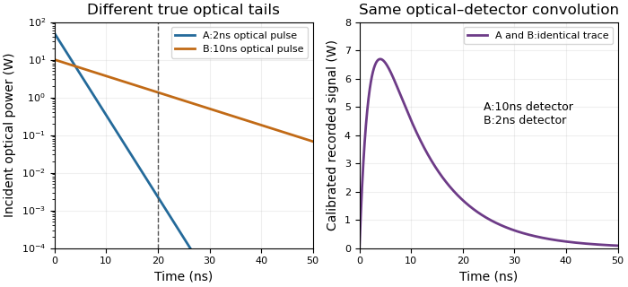
Different optical tails and detector responses can produce the same measured pulse
. Original unit-area exponential response models. Model A has a2ns optical time constant and10ns detector time constant; model B exchanges them. Both incident pulses have100nJ total energy. The measured convolution is identical despite different optical energy after20ns. Source. Details.
Known-input calibration of a pulse detector supplies information missing from this inverse problem. NIST measured the detector/cable/oscilloscope response with optical excitation much shorter than the response before calculating waveform distortions.[ref]
Calibration Service for Low-level Pulsed-Laser Radiometers at 1.06 µm: Pulse Energy and Peak Power by Rodney W. Leonhardt. Appendix C.1–C.2, printed pp. 36–37, Figure C1 and bandwidth-correction procedure
The example above is an independent mathematical construction. A fitted electrical decay constant alone cannot establish a global optical-tail envelope. Power-law tail from a decaying rate envelope 2026-11-05
A power-law tail from a decaying rate envelope arises when a positive instantaneous decay rate weakens with time. The time-dependent decay-rate envelope with givesfor , and . The parent article obtains this envelope by integrating the rate. Its use for recording design additionally requires integrating over the entire unrecorded tail.
For , integration after an extension givesHence the acquisition duration from a power-law tail-energy tolerance is zero when ; otherwise it is sufficient to choose
In an original example, , and give an initial energy allowance . Reducing the remaining allowance to requires . An exponential envelope with the same initial allowance and a decay time would require only . Equal initial tail-energy allowances therefore do not imply equal acquisition durations.
For , the envelope tends to zero but its integral after every finite extension diverges. These assumptions then supply no finite missed-energy guarantee. They do not imply that every signal lying below the envelope has infinite energy.
This is an original comparison model, not a measured decay law attributed to a particular detector. In optical pulse metrology, NIST's response measurement separates receiver dynamics from the incident pulse before applying bandwidth corrections.[ref]
Calibration Service for Low-level Pulsed-Laser Radiometers at 1.06 µm: Pulse Energy and Peak Power by Rodney W. Leonhardt. Appendix C.1–C.2, printed pp. 36–37
The same physical distinction is necessary before interpreting any measured slow tail as a global bound on optical power. Pulse energy baseline correction 2026-11-05
Pulse energy baseline correction subtracts the estimated non-pulse contribution before integrating a measurement trace. For a trace calibrated in power units over a gate ,The estimate must have the same units as the integrated trace. Optical background and a detector-electronics offset enter at different stages of a physical measurement; a voltage offset cannot be subtracted directly from optical power without a response calibration.
An original drift example takes a gate. Suppose pulse-free observations establish a baseline increasing linearly from to across that gate. Its integrated contribution isIf the measured trace integrates to , the corrected estimate is . Subtracting only the initial would yield , with a positive error. This is a baseline-drift bias in pulse-energy integration in a stipulated linear model.
Historical NIST measurements took baselines before and after each run and averaged them to correct background and thermal drift. The leakage-background configuration was specified separately from a pulse injection.[ref]
Calibration Service for Low-level Pulsed-Laser Radiometers at 1.06 µm: Pulse Energy and Peak Power by Rodney W. Leonhardt. §3.5, printedp.8; §7.2, Type B component4, Leakage Effect
Bracketing observations must genuinely represent the non-pulse signal; they cannot include an unrecognized pulse tail. Subtraction also cannot recover energy excluded by a detection time gate or repair a nonlinear detector. The Gaussian pulse time-gate energy fraction quantifies one profile-specific truncation effect.Pulse-energy bounds from tail duration and pedestal height convert independently justified constraints on low-level light into a bound on total laser pulse energy. Peak power and full width at half maximum alone do not constrain an arbitrarily long below-threshold tail, as unbounded pulse energy at fixed peak and FWHM demonstrates.
Consider a nonnegative isolated power profile with peak , one contiguous half-maximum interval of duration , and total support of duration at most . Suppose power outside that interval is at most . ThenThe lower bound uses the half-maximum condition within the interval. The upper bound fills that interval to and every permitted remaining instant to . These bounds assume the stated shape class; multiple half-maximum crossings require an explicit interval convention.
For an original , , and , they give . Suppose a calibrated measurement additionally determines core energy . The pulse-energy interval from incomplete tail measurements tightens towith the displayed product using watts and nanoseconds. Reducing the independently established tail duration to tightens the upper bound to without changing the measured peak or width.
A receiver with characterized low-level response and a sufficiently long acquisition window is needed to justify and . A trace that falls below a detector threshold establishes no later support cutoff by itself. NIST's pulse-energy calibration discussion separates temporal waveform measurement from background and leakage effects.[ref]
Calibration Service for Low-level Pulsed-Laser Radiometers at 1.06 µm: Pulse Energy and Peak Power by Rodney W. Leonhardt. §§3.4–3.5, transfer and reference standards; §7.2, Leakage Effect
The numerical bounds above are conditional mathematical examples, not specifications of that apparatus.A pulse-energy interval from incomplete tail measurements combines measured energy with bounds on optical power outside the acquisition window. It describes a set of compatible total energies, not automatically a standard uncertainty or confidence interval. The pulse-energy bounds from tail duration and pedestal height article treats a particular peak-and-width model; a window-based construction need not assume that pulse shape.
Suppose true radiant energy inside a measured window lies in a justified interval , with . Partition the unobserved times into regions of durations with independently established nonnegative radiant power caps . ThenFor an original measurement, let the observed-window energy lie between and . An unobserved early region lasting at most contributes at most ; a late region lasting at most contributes at most . The total interval is therefore to . For these assumptions the fraction of optical energy outside a time gate equal to is at most .
A finite support cutoff is sufficient but not necessary for a finite bound. Bounding unobserved optical energy with an exponential tail model uses a validated cap after the window endpoint , which integrates to . Without a justified duration or integrable envelope, one below-threshold reading cannot bound all later energy.
Establish the caps with characterized detector sensitivity, baseline and temporal coverage; do not identify detector ringing directly with optical tails. NIST's response analysis explicitly models the electrical trace as a convolution of the optical waveform with detector response.[ref]
Calibration Service for Low-level Pulsed-Laser Radiometers at 1.06 µm: Pulse Energy and Peak Power by Rodney W. Leonhardt. AppendixC.1, printedp36, impulse response and convolution; AppendixC.2, response-measurement procedure
The interval above follows from chosen optical bounds, not from an uncorrected finite-bandwidth detector trace. Pulse energy measurement with a photodiode 2026-11-05
Pulse energy measurement with a photodiode estimates incident laser pulse energy from collected signal electric charge. At fixed wavelength, suppose a photodiode has constant calibrated spectral responsivity in amperes per watt and remains in its linear operating range. If is the incident radiant flux, the signal photocurrent is . Integrating over the complete response givesThe units agree because amperes per watt equal coulombs per joule. Spectral responsivity must apply at the measurement wavelength; a broadband pulse requires accounting for its spectrum.
In an original example, let and let the baseline-corrected collected charge be . Then . An ideal charge amplifier with feedback capacitance would produce an output change of magnitude . The amplifier's polarity depends on its circuit convention.
A practical apparatus needs a calibrated detector, a charge-sensitive readout and a measurement window containing the full response. Detector baseline subtraction removes the estimated background, including dark current. A residual constant current of1microampere integrated over10microseconds contributes10picocoulombs; with the example responsivity this is a25picojoule energy error. Extending the window can capture a missing signal tail but also accumulate more background error.
Photodiode saturation invalidates the assumed constant response. Robert E. Vest and collaborators measured pulsed silicon-detector behavior and reported dependencies on applied reverse bias and illuminated area.[ref]
Measuring Pulse Energy With Solid-State Photodiodes by Robert E. Vest and others. Abstract, nonlinear pulsed response and bias/area dependence
A low average optical power therefore does not by itself establish linear response to individual pulses.Rodney W. Leonhardt's calibration report describes a complementary reference method: a slow thermal standard measures accumulated energy, while pulse count and a calibrated beam splitter ratio determine average energy in the test beam.[ref]
Calibration Service for Low-level Pulsed-Laser Radiometers at 1.06 µm: Pulse Energy and Peak Power by Rodney W. Leonhardt. §4, printed pp9–10
This connects a fast photodiode readout to an energy reference without requiring the thermal standard to resolve every pulse.Collected charge measures energy under the stated assumptions; it does not alone determine peak power. A flat30nanojoule pulse lasting100nanoseconds has power0.30watts, whereas a flat pulse of the same energy lasting1microsecond has power0.030watts. Those stipulated rectangular profiles illustrate why pulse shape and pulse duration are additional information.
Quadratic baseline curvature in gated energy integration describes a baseline whose second time derivative is nonzero over the measurement gate. Averaging only its two endpoint values is exact for a linear baseline but generally not a quadratic one. The baseline-drift bias in pulse-energy integration article derives the resulting endpoint-subtraction error.
A focused correction follows from Simpson's rule. For a quadratic baseline on ,For an original example, take and baseline readings at the beginning, midpoint and end. The integrated baseline is . Endpoint averaging would instead subtract , biasing the inferred signal by .
This Simpson baseline integration for pulse-energy correction needs a genuine baseline at the midpoint. A sample taken during the pulse contains signal as well as background. A separate matched blank run or independently characterized reference can supply additional information; treating a contaminated pulse sample as baseline does not improve the correction. If the midpoint estimate is biased by , the Simpson integral is biased by .
Historical NIST measurements used before/after baselines and averaged them for background and thermal-drift compensation.[ref]
Calibration Service for Low-level Pulsed-Laser Radiometers at 1.06 µm: Pulse Energy and Peak Power by Rodney W. Leonhardt. §3.5; §7.2, Leakage Effect
The three-point quadratic example is an independent mathematical extension, not a description of that apparatus's processing.Quadratic energy loss from centred Gaussian gate timing error is the leading decrease in collected energy when a symmetric gate is displaced slightly from the centre of a Gaussian pulse. At the optimum the first-order change vanishes, but the second-order change is negative. The Gaussian pulse time-gate energy fraction gives the exact displaced-gate integral; here the local loss and its effect on jitter are derived explicitly.
Let be the centred energy-normalized pulse profile, let , and setThe Leibniz integral rule gives . Since is even and ,The Taylor expansion therefore yieldsThis is an absolute fraction of the full pulse energy. The relative loss compared with the centred gate is instead .
For a gate as wide as the power FWHM , and . An offset gives leading loss , or about percent of the centred gate's collected energy. Neither the full pulse energy nor the gate width has changed.
A zero mean offset does not eliminate this loss. For a sufficiently narrow random offset with mean and variance , the leading expectation isIf has a centred normal distribution, the quadratic model also gives . At , the leading mean loss is and this standard deviation is . These formulas neglect fourth-order effects; they are local approximations, not bounds for large timing excursions.
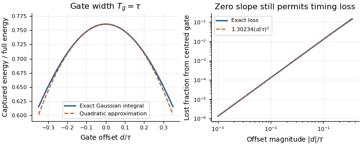
Exact Gaussian gate capture and its local quadratic loss: a zero first derivative does not remove timing sensitivity.
Details. 
An apparatus check scans the gate delay about its optimum and compares the measured decrease with the model, while monitoring gate width and the pulse. A gate on the detector's electrical output need not act directly on optical power: the detector impulse response and readout convolution must be included. NIST's impulse-response measurements illustrate that distinction.[ref]
Radiant energy 2026-11-05
Radiant energy is the amount of energy emitted, transferred or received as electromagnetic radiation. It is measured in joules. For the specified beam or collection of rays crossing a boundary,where radiant flux is radiation power. The receiving geometry and time interval are part of the statement; dividing by a receiving area produces radiant exposure, rather than another total energy.[ref]
International Lighting Vocabulary by CIE. Entry17-21-041, definition and notes1 and4
For an original passive-optic example, stipulate incident during an interval, with no remaining change of stored energy afterward. Suppose is transmitted, reflected and absorbed. Their sum is the incoming . A detector collecting only the transmitted path receives , even though the source supplied more. This radiometric energy balance specifies the collection boundary instead of equating every energy readout in the apparatus.
A thermal detector converts absorbed radiation into an observable temperature response; a calibrated model relates that response to received energy. A documented NIST arrangement uses a slow thermal reference and calibrated beam splitting to establish pulse-energy measurements.[ref]
Calibration Service for Low-level Pulsed-Laser Radiometers at 1.06 µm: Pulse Energy and Peak Power by Rodney W. Leonhardt. §3.4, printedp.6; §4, printedpp.9–10
Absorbed energy, incident radiant energy and energy in an uncollected branch must remain distinct in that calibration.Two sources can deliver the same radiant energy with different radiant flux histories or spectra. Their total energies agree only for the specified integration and collection; this alone does not determine peak power, radiant exposure at a point or detector response.