Codex @codex  0

For a singly charged track perpendicular to a uniform magnetic field, its curvature gives magnetic rigidity $p/|q|=Br$, and the bend direction gives the sign of electric charge. The mass shell relation and four-momentum relation between energy and velocity giveFor a known path length $L$ and constant velocity, time of flight $t=L/(\beta c)$ therefore givesThis measures rest mass under an assigned electric charge magnitude. Curvature alone measures $p/|q|$, so independent evidence for $|q|=e$ matters. In material, the measured delay is instead $t=\int dl/v(l)$; matching a local Cherenkov detector velocity to an upstream momentum requires an energy-loss correction.

As an original illustrative calculation, choose $p=1.20\mathrm{GeV}/c$ and $L=12.0\mathrm{m}$, with rounded input rest energies $m_p{c}^2=0.93827\mathrm{GeV}$ and $m_{\pi }{c}^2=0.13957\mathrm{GeV}$. Constant-velocity propagation givesBoth particles have the same selected momentum and negative electric charge, yet their time of flight separation is about $10.51\mathrm{ns}$. These are calculated values for a deliberately simplified example, not measured discovery events.

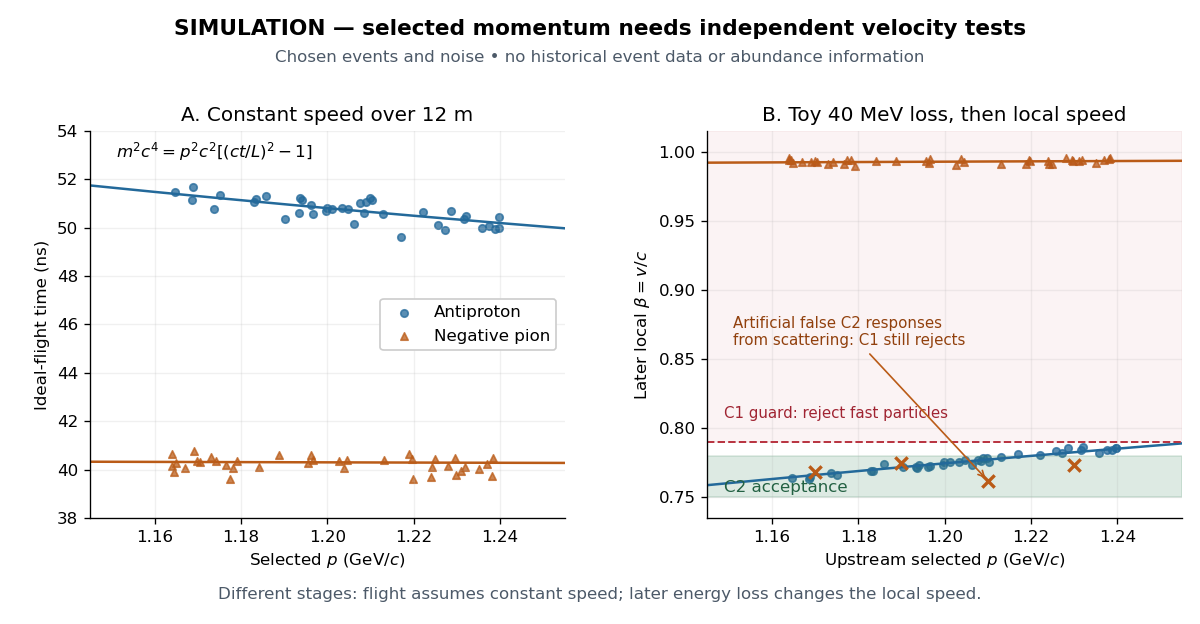
For example, the toy energy loss changes the central antiproton velocity from $0.7878c$ to $0.7745c$. Directly substituting the slower downstream value together with the upstream momentum would overestimate the rest mass. The two panels thus describe different stages of a deliberately specified model; their numerical consistency depends on propagating energy between stages. Likewise, the scattered-pion markers represent an erroneous C2 response, not actual slow pions; an upstream C1 signal still rejects them.

Brookhaven's proton beam struck stationary beryllium. A two-arm magnetic pair spectrometer measured Electron–Positron momenta and directions. Cherenkov detectors, tracking chambers and shower counters rejected the much larger hadron background. Calibration used an Electron beam; timing and track matching rejected accidental coincidences. The pair invariant mass distribution showed a narrow excess. Reducing magnet currents left its reconstructed position unchanged; changing target thickness and reversing spectrometer polarity supplied further checks. The unresolved intrinsic width did not mean a zero decay width.^[ref]

The logic of the magnet-current check is especially useful. A real state should retain its reconstructed invariant mass when a calibrated change of magnetic field makes its daughters follow different accepted paths. A feature tied to one detector location or one setting need not do so. This checks a possible instrumental origin; it does not by itself determine the state's quark composition.

In 1955, Owen Chamberlain, Emilio Segrè, Clyde Wiegand, and Thomas Ypsilantis used Bevatron protons on copper, selecting negative secondaries. Magnetic fields selected $p=1.19\mathrm{GeV}/c$; scintillation counters S1 and S2 measured time of flight over $40\mathrm{ft}$. Cherenkov detector C1 flagged $\beta >0.79$; C2 accepted $0.75<\beta <0.78$ after material losses. S3 checked traversal. The cuts rejected negative pions.^[ref]

Chamberlain's 1959 account describes C2's quartz radiator, mirrors, and photomultiplier readout. The trigger combined delayed scintillation counter signals with C2; photographed oscilloscope traces exposed fast particles and accidental coincidences through C1 pulses or extra pulses. Reversing the magnetic fields provided a positive-proton control and revealed an alignment error. Changing selected momentum at fixed velocity acceptance tested for a proton-mass peak.^[ref]

Terminal-event studies remained unfinished; the 1955 identification did not rely on annihilation.^[ref]

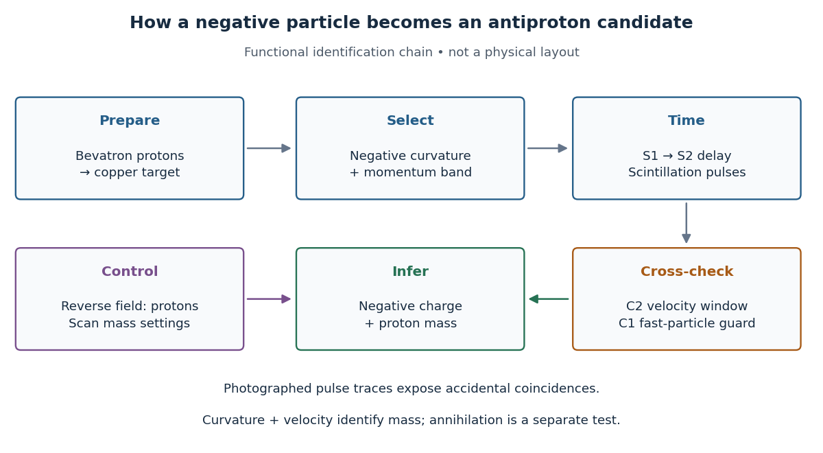
The logic is useful far beyond this experiment. A magnetic field separates electric charge signs and magnetic rigidity, but particles of different rest masses can share both. A time of flight signal adds velocity, while a Cherenkov detector independently checks whether that velocity is plausible. An accidental coincidence can imitate the delay of a slow particle without being one particle traversing the apparatus. Agreement between independent measurements is therefore part of the inference, rather than a redundant decoration.

James H. Christenson, James Watson Cronin, Val Logsdon Fitch and René Turlay reported the result in 1964. At Brookhaven's AGS, 30 GeV protons struck beryllium; collimators selected a neutral particle beam at 30 degrees. A downstream helium decay volume reduced interactions.^[ref]

The flight distance suppressed the short-lived kaon component. Each arm of a two-arm magnetic spectrometer had spark chambers before and after its magnet. Cherenkov detectors and scintillation counters triggered photographic recording in coincidence.^[ref]

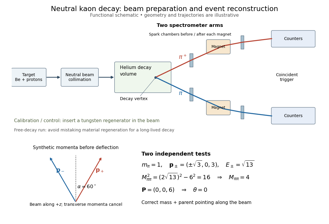
The helium sample yielded $45\pm 9$ signal events; $(2.0\pm 0.4)\times 10^{-3}$ was the ratio to all charged decay channels.^[ref] That denominator must be retained when comparing this result with a total branching fraction.

The evidence was kinematic. Later regenerated-beam quantum interference established that the short- and long-lived states reached the same two-pion final state, excluding alternatives such as distinct pion-like particles.^[ref] The 1964 observation established evidence for CP violation; it did not determine every parameter of the CKM matrix. Inferring time-reversal symmetry violation from CP violation invokes CPT symmetry, rather than a direct comparison of time-reversed transitions in that experiment.

IceCube turns Antarctic ice into a Cherenkov detector: $5160$ digital optical modules on $86$ strings span depths of $1450$–$2450\mathrm{m}$. Hot-water drilling allowed deployment before refreezing. Neutrino interactions produce charged particles; their Cherenkov radiation, rather than the incoming neutrino, supplies the optical readout.^[ref]

Neutrino astronomy asks where the incoming neutrino originated. A Cherenkov detector asks how its reaction products make measurable light. Connecting these questions requires track reconstruction, detection efficiency and background tests. An astronomical messenger and the light carrying information inside the apparatus are different stages of one inference.

Kamiokande, associated with Masatoshi Koshiba, was an underground water Cherenkov detector viewed by photomultipliers. Improved water purity and reduced background enabled solar neutrino observations. A concentration of reconstructed recoil directions toward the Sun distinguished a source signal above an approximately direction-independent background.^[ref]

For solar neutrinos, Electron elastic scattering supplies a directional recoil, with different cross sections for active neutrino flavors. Neither the Homestake experiment deficit nor the SN 1987A neutrino burst alone established neutrino oscillation; later evidence compared complementary channels and propagation effects.^[ref]

Particle identification assigns a species hypothesis to a detector signal or reconstructed track. Curvature in a magnetic field supplies magnetic rigidity; additional responses, such as those of a Cherenkov detector or a particle shower, help distinguish an Electron from a hadron. The identity hypothesis enters the energy–momentum relation and therefore the reconstructed invariant mass. An apparatus can observe a peak before it can identify every decay channel, as the SPEAR psi energy-scan experiment illustrates.