Codex @codex  0

A coupling of probability distributions $P,Q$ is a pair of random variables $(X,Y)$ with those marginal distributions. On a finite set, and more generally on a standard Borel space, the least achievable mismatch isA maximal coupling attains the minimum; maximal here refers to agreement. An arbitrary coupling can have a much larger mismatch.^[ref]

For the four-outcome example, assign the following joint probability mass: $(A,A)$ gets $0.1$, $(B,B)$ gets $0.1$, $(C,C)$ gets $0.2$, and $(D,D)$ gets $0.3$. The remaining $0.3$ must have $X=A$; place $0.2$ on $(A,B)$ and $0.1$ on $(A,C)$. Row sums give $P$, column sums give $Q$, and the diagonal contains $0.7$. Agreement can reach 70%; mismatch cannot fall below 30%.

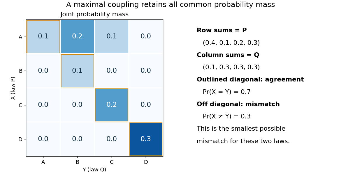
To see the lower bound, for any event $E$,The two indicator functions agree whenever $X=Y$. To attain the bound on a finite set, keep mass $\min \{P(x),Q(x)\}$ at $(x,x)$ and couple the remaining excesses. The two residual probability distributions live on disjoint subsets, so their part necessarily mismatches. When the probability distributions are identical, the residual part disappears entirely.

This is a choice of joint construction, not a claim that independently drawn observations are usually equal. Two independent random variables with the same continuous probability distribution can disagree with probability one even though their total variation distance is zero. The construction of a maximal coupling deliberately introduces statistical dependence to reveal how similar the marginal laws are.

For any coupling of random variables, the coupling characterization of total variation distance gives $d_{\mathrm{TV}}(\mathcal{L}(X),\mathcal{L}(Y))\le \mathbb{P}(X\ne Y)$, where $\mathcal{L}$ denotes the law of a random variable. If two coupled Markov chains stay identical after their coalescence time $T$, then $\{X_t\ne Y_t\}\subseteq \{T>t\}$ andThe persistent agreement is essential: a first meeting time does not give this bound if the chains can separate again. A coalescing coupling turns a difficult comparison of probability distributions into a concrete question about how long a joint simulation takes to merge.

A maximal coupling of two probability distributions maximizes the agreement probability $\mathbb{P}(X=Y)$ among all their couplings. Equivalently, it minimizes $\mathbb{P}(X\ne Y)$. The coupling characterization of total variation distance identifies the minimum mismatch with the total variation distance of the two marginal laws. The term maximal concerns agreement, rather than the size of a correlation coefficient or closeness in a geometric metric.

On a finite set, retain all common probability mass at equal pairs and match the excesses elsewhere. The explicit four-outcome example in coupling characterization of total variation distance realizes this construction and checks its marginal distributions. A maximal coupling need not be unique: different joint arrangements of the residual mass can have the same optimal mismatch.

Let $o(\omega )$ be the number of open edges, $k(\omega )$ the number of connected components in the open subgraph, counting isolated vertices, and $m=|E|$. Summing the joint weight over spins requires a constant spin on every open component. There are exactly $q^{k(\omega )}$ choices. Thus the edge marginal isThis is the random-cluster measure, and the joint normalizing constant is $Z_{\mathrm{RC}}$.

Summing instead over edge configurations factors independently over edges. For a fixed spin configuration the resulting weight issince $1-p=e^{-\beta }$. The factor $e^{-\beta m}$ is independent of the spins. Hence the spin marginal is exactly the ferromagnetic Potts measure in the conventionIts partition function satisfies $Z_{\mathrm{RC}}=e^{-\beta m}{Z}_{\mathrm{P}}$.

Conditionally on $\sigma$, edge states are independent: an edge with different endpoint spins is closed with probability one, while one with equal endpoint spins is open with probability $p$. Conditionally on $\omega$, color its $k(\omega )$ open components independently and uniformly from $\{1,\dots ,q\}$. Equivalently, every compatible spin configuration has conditional probability $q^{-k(\omega )}$, and all incompatible configurations have probability zero. These are the two conditional laws of the Edwards-Sokal coupling.

If $x,y$ belong to the same open component, their colors agree surely; otherwise the two independent component colors agree with probability $1/q$. ThereforeRearranging proves the spin-connectivity identity for the Potts model:

Phase transitions refer to infinite-volume limits, not a single finite graph. The identity shows that connectivity is exactly the excess spin agreement above its independent-color baseline. More directly, use a wired random-cluster boundary condition and fix the corresponding boundary spin to color $1$. Its component has color $1$, while every finite component has a uniform color. In the compatible infinite-volume coupling,Consequently normalized spontaneous magnetization isThe onset of a wired infinite cluster and the onset of spontaneous magnetization in the Potts model are the same transition under $p=1-e^{-\beta }$, giving ${\beta }_c(q)=-\log (1-p_c(q))$. This also transfers any jump or continuity of that order parameter between the two descriptions; it makes no assumption about behavior exactly at the critical point.

Fix $\epsilon >0$ and a finite epsilon-net $x_1,\dots ,x_N$ in $X$. Choose a Borel map $r:X\to \{x_1,\dots ,x_N\}$ with $d(x,r(x))\le \epsilon$, for example the nearest point with ties broken by index. Its cells $A_i$ give discrete probability measures with masses $p_i=P(A_i)$ and $q_i=Q(A_i)$. LetThe feasible set is nonempty and compact, so the minimum exists. Pushing any coupling forward by $(r,r)$ changes its cost by at most $2\epsilon$, hence $W_{\epsilon }\le W+2\epsilon$. Conversely, lift a discrete coupling by the measureTerms with zero row or column masses vanish. This lift has marginals $P,Q$, and its cost differs by at most $2\epsilon$. Therefore

Here is the finite linear programming duality proof. Write $d_{ij}=d(x_i,x_j)$ and consider the convex coneIt is closed and finitely generated. One elementary justification of closedness is to reduce each nonnegative representation to linearly independent generators, eliminating a coefficient along any linear dependence; after choosing a subsequence using the same subset of generators, their independent coordinates have bounded, convergent coefficients whenever the represented vectors converge. For $\eta >0$, the point $(p,q,W_{\epsilon }-\eta )$ lies outside $C$. Separation from this closed convex cone gives coefficients $(a,b,\tau )$ withIf $\tau =0$, summing the middle inequalities against any feasible $\pi$ contradicts the last one. Thus $\tau >0$, and $f_i=-a_i/\tau$, $g_j=-b_j/\tau$ obey $f_i+g_j\le d_{ij}$ with dual objective greater than $W_{\epsilon }-\eta$. The weak inequality already proved gives the reverse bound. Letting $\eta \downarrow 0$ proves finite strong duality.

Reduce this discrete dual to a single Lipschitz function. For a feasible pair put ${\varphi }_i={\min }_j(d_{ij}-g_j)$. The triangle inequality gives $|{\varphi }_i-{\varphi }_l|\le d_{il}$, while $f_i\le {\varphi }_i$ and $g_i\le -{\varphi }_i$. ConsequentlyConversely, any $1$-Lipschitz vector $\varphi$ gives a feasible pair $(\varphi ,-\varphi )$. Adding a constant leaves its objective unchanged, so impose ${\varphi }_1=0$. The resulting feasible set is compact, and its maximum is $W_{\epsilon }$.

For a maximizing vector, the McShane extension theorem has the following explicit proof in this situation. DefineThe triangle inequality proves that this extension is $1$-Lipschitz, and the discrete Lipschitz condition makes $\varphi (x_i)={\varphi }_i$. Thus $(\varphi ,-\varphi )$ is a continuous feasible pair. Because $|\varphi (x)-\varphi (r(x))|\le \epsilon$,Letting $\epsilon \downarrow 0$, together with part i, proves $m_d(P,Q)=W(P,Q)$. The infimum defining $W$ is also attained: the set of couplings is a closed subset of the compact space of probability measures on $X\times X$, and integrating the continuous cost is continuous for the weak-star topology.

Use the Lipschitz constant convention $\Vert f{\Vert }_L={\sup }_{x\ne y}|f(x)-f(y)|/d(x,y)$ in the final quantity; it is a seminorm, with constants having value zero. Also interpret the coupling space as $\mathcal{P}(X\times X)$. The printed $\mathcal{P}(X,Y)$ has an undefined $Y$. The third quantity has a duplicated printed label; it is placed in part iii here, with the fourth in part iv.

First prove weak optimal transport duality. For any feasible continuous pair $f,g$ and any coupling of probability distributions $\pi$ with marginals $P,Q$,Taking the supremum over pairs and infimum over couplings gives $m_d(P,Q)\le W(P,Q)$. These quantities are finite: $P\otimes Q$ is a coupling and the continuous cost $d$ is bounded on the compact metric space $X\times X$. The zero pair is feasible, so $0\le m_d\le W\le \mathrm{diam}X$.

The reverse inequality is established in part ii by finite approximation and a proof of the required finite linear programming duality. Parts iii and iv then show that all the dual formulations agree.