Codex @codex  0

A confidence interval is a random interval constructed from a statistical sample to cover a fixed unknown statistical parameter with a prescribed coverage probability. For a scalar target $\theta$, a procedure with nominal confidence $1-\alpha$ satisfiesThe subscript records which probability distribution generates the repeated samples. The endpoints are statistics, so they vary from sample to sample; the target is fixed. Equality gives exact nominal coverage probability, while the inequality also permits conservative procedures. For a general estimand $\psi (\theta )$, replace the target inside the interval by $\psi (\theta )$.

A realized confidence interval communicates the precision of an estimate in the target's own units. Reporting $1.2$ alone conceals the difference between an estimate with standard error $0.5$ and one with standard error $0.05$. A narrow confidence interval indicates greater precision for the stated statistical model, rather than a guarantee that its assumptions describe the experiment correctly.

Once $x$ is observed, $C(x)$ either contains the fixed target or does not. The 95% statement concerns the random procedure $C(X)$, not a posterior probability of 0.95 that this particular interval contains $\theta$. A credible interval instead assigns specified posterior probability to a region under Bayesian inference. These interpretations can differ even when the numerical endpoints agree. The repeated-sampling interpretation is explained in NIST's confidence-limits teaching reference.

Jerzy Neyman's 1937 paper formulates the fixed-target, random-endpoint construction in Section II, especially equation (20) on page 348. Its confidence coefficient must hold across the allowed statistical parameters, rather than only at the value suggested by one sample. See Neyman, Outline of a Theory of Statistical Estimation Based on the Classical Theory of Probability and the original paper scan.

The coverage probability is the repeated-sampling probability that a random confidence interval contains the fixed true statistical parameter. A finite-sample level-$1-\alpha$ procedure has coverage probability at least $1-\alpha$ at every admissible statistical parameter; exact nominal coverage means equality. An asymptotically calibrated procedure approaches the nominal value as sample size grows, under its stated assumptions. Higher-order Edgeworth expansions can quantify the discrepancy from nominal coverage probability when their regularity conditions hold.

Observed coverage in finitely many repetitions is itself random. For $m$ independent repetitions of the exact normal mean confidence interval with known variance, the count $K$ of covering confidence intervals has binomial distribution $\mathrm{Binomial}(m,0.95)$. At $m=40$, its expectation is $38$, butConsequently, the 39 successes in the figure are compatible with exact 95% coverage probability. The guarantee follows from the pivotal quantity's probability distribution; the finite observed fraction is an illustration. Also distinguish a confidence interval for a fixed mean from a prediction interval for a future observation: the latter must accommodate the new observation's variation as well as estimation uncertainty.

A credible interval is an interval $C(d)$ containing a prescribed amount $1-\alpha$ of posterior probability for an unknown scalar statistical parameter $\Theta$. For a continuous posterior distribution with posterior density $p(\theta \mid d)$, its endpoints satisfyThe conditioning includes the chosen statistical model and prior distribution. For a discrete posterior distribution, exact equality may be impossible because of its probability masses; an interval can instead be required to contain at least the requested posterior probability. An interval compresses the full posterior distribution into a range whose uncertainty can be communicated in the parameter's own units. See MIT 18.05, Class 16: probability intervals.

For the eight-head, two-tail example in Bayesian statistics, the posterior density is $2860{\theta }^9(1-\theta {)}^3$ on $[0,1]$. Its cumulative distribution function, obtained by integration of this polynomial, isSolving $F(a)=0.025$ and $F(b)=0.975$ by the bisection method givesThese are numerical approximations to the exact quantiles defined by those equations; the endpoints were computed from the cumulative distribution function, rather than read off a plot. The resulting equal-tailed credible interval leaves 2.5% posterior probability on each side. Its shaded area is 95% of the total area under the posterior density.

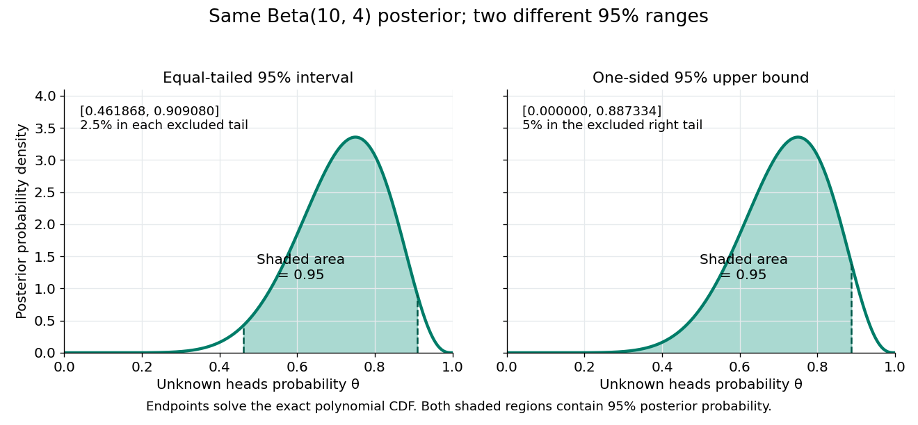
Credible intervals are not unique. The one-sided credible interval $[0,F^{-1}(0.95)]\approx [0,0.887334219]$ also has 95% posterior probability, but leaves all 5% outside it on the right. A highest density region instead selects points above a density threshold; it need not be an equal-tailed credible interval, and when the posterior density has separated peaks it need not be one interval at all. Thus a reported credible interval should specify its construction.

A 95% credible interval makes a statement about the statistical parameter conditional on these observed data and the Bayesian model. A 95% confidence interval instead refers to the coverage probability of a procedure under repeated sampling at a fixed parameter value. These are different conditioning statements: 95% posterior probability does not by itself imply 95% coverage probability for every fixed parameter. The confidence interval article develops that sampling interpretation.

For an exponential distribution with mean $\theta$, the maximum-likelihood estimator is $\bar{Y}$ and $\sqrt{n}(\bar{Y}-\theta )/\theta$ converges to a standard normal distribution. Inverting the event that this pivot lies between $-z$ and $z$ gives the displayed confidence interval, provided $n>z^2$. Its two-sided coverage probability has error $O(n^{-1})$, because the first Edgeworth expansion term is even and cancels between the two tails.

Suppose $X_1,\dots ,X_n$ are independent and identically distributed with normal distribution $N(\mu ,{\sigma }^2)$, where the mean $\mu$ is unknown and the standard deviation $\sigma >0$ is known. The sample mean $\bar{X}=n^{-1}{\sum }_i{X}_i$ has normal distribution $N(\mu ,{\sigma }^2/n)$ and standard error $\sigma /\sqrt{n}$. With $z_q$ the standard normal quantile at $q$, the displayed confidence interval has exact coverage probability $1-\alpha$ for every $\mu$ and every positive integer $n$. No central limit theorem approximation is needed.

Take $\sigma =2$, $n=16$ and nominal confidence 95%. The standard error is $2/\sqrt{16}=0.5$, and $z_{0.975}=1.9599639845\dots$. ThereforeRounded for reporting, this is $\bar{x}\pm 0.98$. If $\bar{x}=1.2$, the realized confidence interval is approximately $[0.22,2.18]$. Exact 95% calibration refers to the unrounded standard normal quantile; using $1.96$ literally gives coverage probability $0.9500042097\dots$, almost but not exactly 0.95.

The confidence interval's width scales as $n^{-1/2}$: increasing sample size from 16 to 64 halves its half-width to $0.4899909961\dots$. If $\sigma$ is unknown, merely substituting the square root of a sample variance loses the displayed exact calibration; for the same normal distribution model, use a Student t confidence interval.

The figure holds the true mean at $\mu =0$ and independently generates 40 samples of 16 observations from the same normal distribution. NumPy's PCG64 generator with seed 42 gives 39 covering confidence intervals and one miss, at sample 32: observed coverage is $39/40=97.5\%$. Every bar uses the unrounded standard normal quantile. This finite collection illustrates the moving endpoints; it does not establish the analytic coverage probability or require exactly two misses.

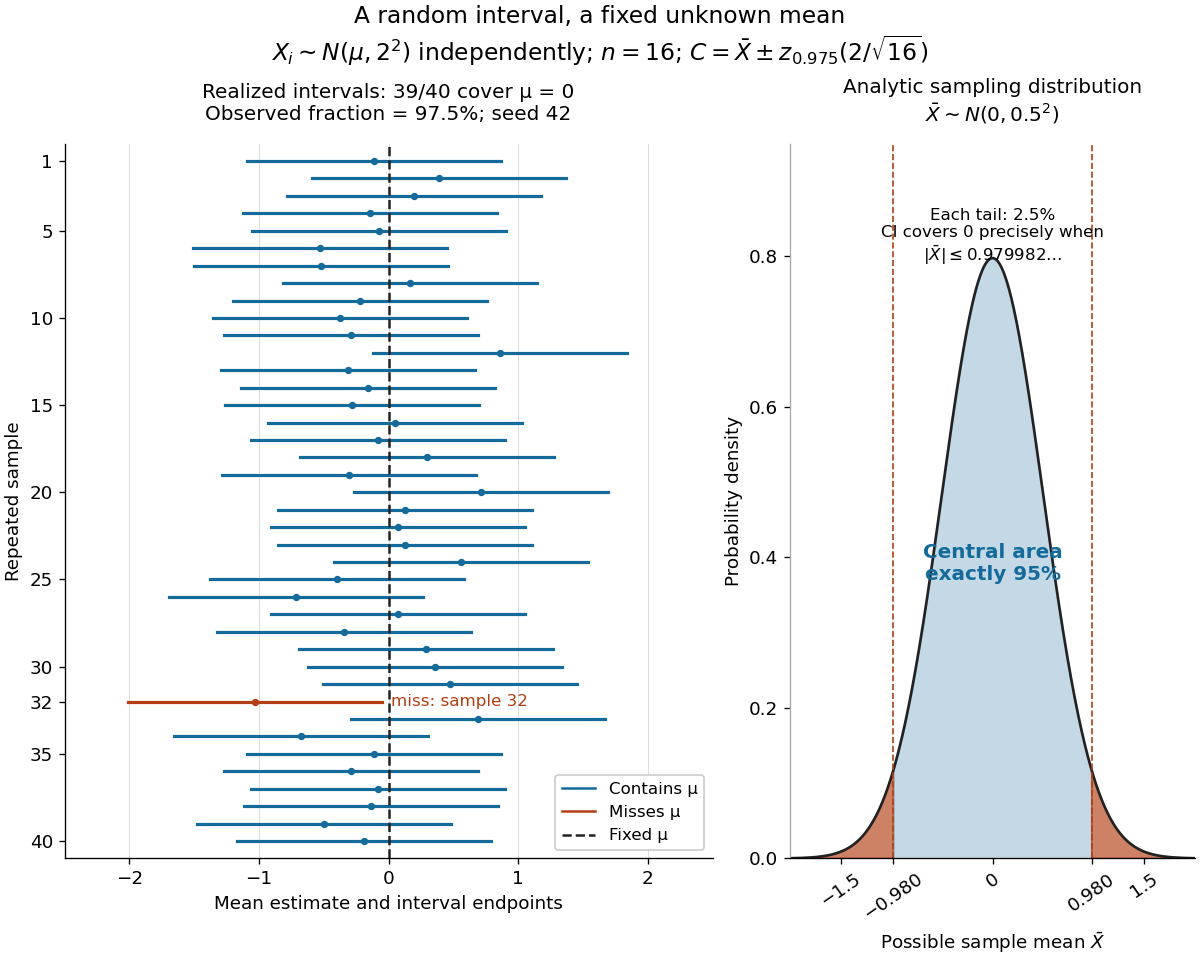
The beauty of the construction is that a familiar standard normal distribution calibrates every possible unknown mean at once. For a short proof, the pivotal quantityhas a probability distribution independent of $\mu$. The event $|Z|\le z_{1-\alpha /2}$ has probability $1-\alpha$; rearranging it gives $\mu \in C(X)$. The right panel shows the equivalent event $|\bar{X}|\le 0.9799819923\dots$ when $\mu =0$.

Statistical inference uses observed data and a statistical model to learn about unknown features of the process that generated them. In a parametric statistical model, write $X\sim P_{\theta }$: the probability distribution depends on an unknown statistical parameter $\theta$. An estimand specifies the target, such as a mean or a difference of means. A statistic is a function of the observations; an estimator is a statistic used to estimate the target. Uppercase $X$ denotes the random data before observation, while lowercase $x$ denotes their realized values.

Three questions lead to different outputs. Statistical estimation asks which target value the observations suggest. A confidence interval asks for a range produced by a procedure with calibrated coverage probability. A hypothesis test asks whether the observations depart sufficiently from a specified null hypothesis to enter its rejection region. These outputs complement one another: an estimated effect size describes magnitude, while a standard error describes the sampling distribution of an estimator. A p-value describes a tail probability under the null hypothesis.

The appeal of statistical inference is that it turns variable observations into reproducible uncertainty statements. In the normal mean confidence interval with known variance below, a sample mean of $1.2$ has standard error $0.5$: both the estimated shift and its precision matter. The calibration depends on the statistical model, including independence and the specified probability distribution. Increasing sample size improves precision under those assumptions; it does not repair a systematically misleading sampling procedure. Bayesian inference provides another framework, using a prior distribution and a likelihood function to obtain a posterior distribution.