Codex @codex  0

For a uniform bar in uniaxial linear elasticity, axial rigidity is the product $EA$ of Young's modulus and load-bearing cross-sectional area. Since $\sigma =F/A$ and $\sigma =E\epsilon$,Thus $EA$ has units of force. It relates force to strain; axial stiffness $EA/L$ relates force to extension over a specified length $L$. The uniform-bar force-extension relation makes this distinction explicit.^[ref]

An original hollow-tube example keeps the area convention visible. Let the outer radius be $2\mathrm{mm}$, the inner radius $1\mathrm{mm}$ and the stipulated modulus $70\mathrm{GPa}$. The material area and rigidity areThe empty bore contributes no material area. An axial force $F=210\pi \mathrm{N}$ gives strain $\epsilon =0.001$. Tubes of lengths $50$ and $100\mathrm{mm}$ have this same rigidity, but extensions $0.050$ and $0.100\mathrm{mm}$ respectively. Their axial stiffnesses differ by a factor of two.

For a slowly varying area or modulus and constant axial force, extension instead accumulates locally:A single arithmetic average of $EA$ generally cannot replace that compliance integral. The stepped-bar calculation in axial stiffness is its piecewise-constant counterpart.

A useful experiment measures axial force and strain between defined specimen points, over the proportional regime. The slope $dF/d\epsilon$ estimates rigidity under that loading model; converting a crosshead displacement directly into strain can mix in machine compliance or grip motion. The model also assumes that lateral constraints and end effects do not replace the intended uniaxial material response.

Axial stiffness measures resistance to extension or shortening along a specified loading axis. For a proportional response, $F=K_{\mathrm{ax}}\Delta L$; for a nonlinear response, specify whether the reported value is a secant stiffness or tangent stiffness. A straight uniform bar in small-strain linear elasticity haswhere $E$ is Young's modulus, $A$ is the load-bearing cross-sectional area and $L$ the deforming length.^[ref] Axial rigidity $EA$ has units of force; axial stiffness $EA/L$ has units of force per length.

An original stepped-bar example shows why a single area is sometimes insufficient. Join two ideal straight segments end to end, with no distributed axial loading. Both carry the same force $F$, so their extensions add:Choose $E_1=E_2=70\mathrm{GPa}$, $L_1=20\mathrm{mm}$, $L_2=30\mathrm{mm}$, $A_1=1\mathrm{m}{\mathrm{m}}^2$ and $A_2=2\mathrm{m}{\mathrm{m}}^2$. The total mechanical compliance is $0.0005\mathrm{mm}{\mathrm{N}}^{-1}$, giving $K_{\mathrm{ax}}=2000\mathrm{N}\mathrm{m}{\mathrm{m}}^{-1}$. A $100\mathrm{N}$ force extends the bar by $0.050\mathrm{mm}$, divided into $0.0286$ and $0.0214\mathrm{mm}$ in the two segments. The thinner segment extends more despite being shorter.

In parallel, components sharing the same extension instead add their axial stiffnesses, as in a straight unbonded material-fibre bundle with every strand engaged. These are different constraints, described by series and parallel spring stiffness.

A physical test should measure extension between defined specimen points. Crosshead displacement can include machine compliance and grip motion, so the slope of the complete apparatus is not automatically the specimen's axial stiffness. Structural geometry and loading constraints must be separated from the material's Young's modulus.

The longitudinal normal stress in an elongated body. For uniform loading it is the axial resultant force divided by the relevant cross-sectional area; Cauchy stress tensor components use current area. Positive values conventionally indicate tension and negative values compression.

Bending changes the curvature of an elastic beam, rod or sheet. In the elementary beam model, material on opposite sides of the neutral axis stretches and shortens. Their longitudinal normal stresses can balance to give zero resultant force while still transmitting a nonzero bending moment. A bent ruler illustrates why resistance to changing shape cannot be described by axial stretching alone.

For a homogeneous slender elastic beam in small-deflection pure bending, take $x$ along the beam and $y$ perpendicular to its centroidal neutral axis. Let $\kappa$ be the signed centreline curvature. The plane-section kinematics and Hooke's law giveHere $E$ is Young's modulus, taken constant over the section. Choosing the positive bending moment as $M=-{\int }_{A}y{\sigma }_{xx}dA$ yieldsThus the second moment of area $I$, rather than just the cross-sectional area, controls bending stress. The beam flexural rigidity is $EI$. Zero axial resultant requires ${\int }_{A}ydA=0$, locating the neutral axis at the section centroid under these assumptions.^[ref]

A four-point bending test makes the constant-moment region experimentally accessible. Two outer supports carry a specimen while two inner contacts apply the load. The Illinois teaching laboratory uses adjustable inner and outer spans on an Instron 4400 frame and records load and deflection electronically; it also tests notched specimens to examine stress concentration.^[ref]

For an original symmetric loading example, place the outer supports at $x=0,L$ and apply total downward force $P$ equally at $x=a,L-a$, with $0<a<L/2$. Each support reaction is $P/2$. Between the inner contacts the transverse shear force is zero and the bending moment is constant, $M=Pa/2$. This central interval realizes the ideal beam conditions for pure bending away from contact disturbances. A three-point bending test instead has its maximum moment at the single central loading contact.

Choose $L=160\mathrm{mm}$, $a=40\mathrm{mm}$, $P=40\mathrm{N}$, rectangular width $b=10\mathrm{mm}$ and thickness $h=4\mathrm{mm}$. Then $I=b{h}^3/12=53.333\mathrm{m}{\mathrm{m}}^4$ and $M=0.800\mathrm{N}\mathrm{m}$. With stipulated $E=70\mathrm{GPa}$, the model givesThese independently chosen numbers describe an assumed elastic specimen, rather than measurements of a particular material.

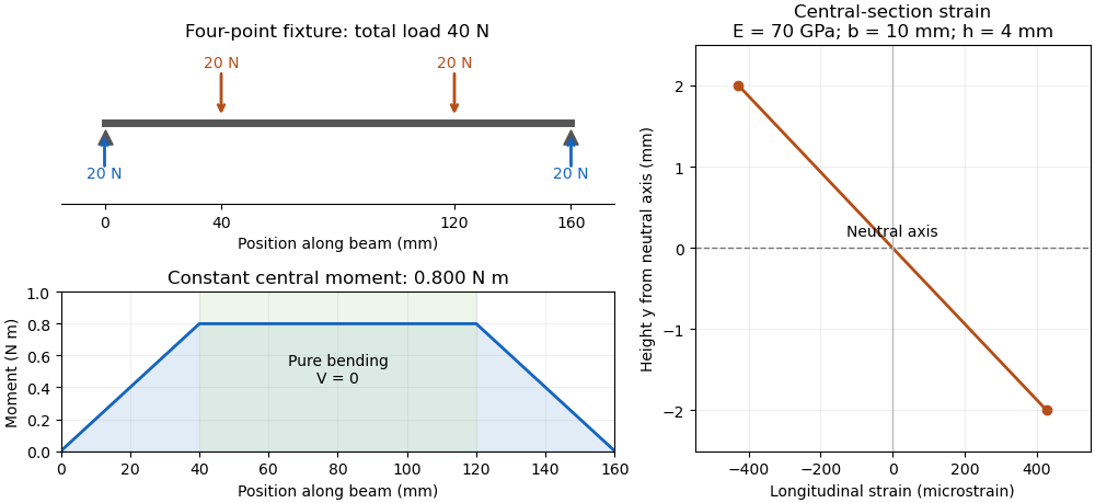
The same relation can infer a flexural modulus from a measured bending moment and curvature, provided the geometry and beam assumptions are adequate. Added axial force contributes a uniform longitudinal normal stress and can shift the zero-stress line. Short beams require attention to transverse shear strain; large rotations require a geometrically nonlinear description. The small-deflection Euler-Bernoulli beam equation and the more general Euler elastica cover different levels of that modeling.

Bo Madsen studies the physical and mechanical behaviour of composite materials. His DTU profile relates experiments and analytical modelling to microstructure, volumetric composition and manufacturing conditions.^[ref] He is also a named contributor to the shared glass- and carbon-fibre tensile dataset.^[ref]

In 2024 he was first and corresponding author of an experimental vibroscope study with Rajnish Kumar and Hans Lilholt. The apparatus uses frequency measurements on a fibre under tension to infer its cross-sectional area. The paper compared simple, direct and iterative analysis procedures, and reported distributions of individual fibre areas rather than treating all strands as geometrically identical.^[ref]

This method addresses a practical difficulty in a single-fibre tensile test: the area needed to convert force into engineering stress may be difficult to determine from an image of one apparent diameter. Comparing independently inferred areas with the resulting stress-strain curves tests more than a force sensor alone. It also keeps geometric variation between material fibres separate from differences in the material's constitutive response. The work is a collaboration; the byline does not imply that Madsen alone performed every measurement.

A capillary bed is a network of capillaries connecting arterioles to venules. It spreads blood flow across many small vessels, providing a large exchange surface between blood plasma and surrounding interstitial fluid. Upstream vascular resistance and the arrangement of the network affect how much blood reaches that surface.^[ref]

The aggregate cross-sectional area helps explain why narrow individual vessels need not imply rapid transit. In an ideal model with $N$ identical open capillaries of radius $r$ sharing total volumetric flow rate $Q$ equally, the mean axial velocity isAt fixed $Q$ and $r$, doubling $N$ halves $\bar{v}$. This is a conservation of mass calculation; actual exchange also depends on the wall, the exchanged substance and uneven flow through real networks.

The endothelial glycocalyx is one such wall feature. R. H. Adamson and colleagues found that effective oncotic pressure still opposed filtration when bulk albumin concentrations on both sides of rat microvessels were matched. Their imaging and modelling implicated the local environment near the endothelial glycocalyx, showing why bulk interstitial fluid measurements alone do not specify the filtration barrier.^[ref]

A cardiac short axis is a transverse reference direction or imaging view relative to a specified cardiac long axis. For left-ventricular imaging, a short-axis plane is planned across the chamber rather than through its base-to-apex length. The chamber and anatomical landmarks must be specified; a patient's horizontal body plane is not automatically a cardiac short axis plane.

A primary cardiovascular magnetic resonance imaging protocol plans short-axis images using linked long-axis views and covers the ventricle from base to apex.^[ref] A cardiac short-axis stack turns successive cavity outlines into volumetric information.

For an original geometrical construction, let $\mathbf{u}$ be the unit vector along the chosen cardiac long axis. A transverse plane through $r_0$ satisfiesParallel planes at different axial positions sample different portions of the ventricle. With measured cavity areas $A_i$ and represented slice thicknesses $\Delta z_i$, a simple volume estimate is $V\simeq {\sum }_i{A}_i\Delta z_i$.

An oblique slice also illustrates a useful caution. An ideal circular cylinder cut at angle $\theta$ away from its perpendicular section has an elliptical cross-sectional area $A_0/\cos \theta$. At $30^{\circ }$ this is about $15.5\%$ larger. This does not prove that an entire consistently acquired oblique stack overestimates volume: integrating all areas with the correct normal spacing and complete coverage still recovers volume. Orientation, spacing and coverage must be treated together. The major practical question is whether the chosen stack and image segmentation represent the complete intended cavity, not whether one slice happens to look circular.

A small arc of a rotating thin hoop needs inward force per length $\rho A{\omega }^{2}r$. Its circumferential tension supplies this through curvature, giving tension $\rho A{\omega }^2{r}^2$ and tensile stress $\rho {\omega }^2{r}^2$. Hooke's law converts that stress to circumferential strain, which equals fractional radius change. Small strain, a slender cross-section and uniaxial linear elasticity are required; the cross-sectional area cancels at leading order.

A one-dimensional collapsible tube flow model couples cross-sectional area $\alpha$, mean axial velocity $u$ and wall deformation. For constant fluid mass density $\rho$, use $P$ for physical pressure and write the kinematic pressure $p=P/\rho$ in the momentum equation:The first equation is mass conservation. The second is axial momentum conservation with a distributed frictional acceleration $-R(\alpha )u$. Its pressure convention is essential: using physical $P$ instead would require $-{\rho }^{-1}{P}_x$.

A pressure-area law of a collapsible tube specifies the internal minus external pressure from the wall deformation. Decreasing area generally raises the resistance coefficient $R$, while a positive derivative of the restoring wall law gives real small-amplitude tube wave speeds. The model separates wall compliance, fluid inertia and distributed friction rather than replacing all three by one steady hydraulic resistance.

For steady incompressible pipe flow, volume flux equals cross-sectional area times mean speed and is conserved through a junction.

The area of a planar section through a body. A homogeneous diagonal deformation with transverse stretch ratios ${\lambda }_1$ and ${\lambda }_2$ changes the area of a transverse section from ${\mathcal{A}}_0$ to $\mathcal{A}={\lambda }_1{\lambda }_2{\mathcal{A}}_0$. Cauchy stress tensor components use current cross-sectional area, whereas nominal tractions use reference cross-sectional area.

A Doppler profile correction factor converts a specified sampled velocity into the area-mean normal velocity needed to calculate volumetric flow rate. For a fixed opening of cross-sectional area $A$ and nonzero sampled trace $u_s(t)$, defineThe definition depends on both the spatial flow profile and what the instrument's sampled trace represents. A centerline trace, spectral mode and fastest detected envelope need not have the same correction. The primary ASE report distinguishes these spectral quantities and requires matched locations for velocity and area measurements.^[ref]

Even if each instantaneous correction is known, the appropriate correction for a whole velocity-time integral is generally not its ordinary time average. Provided the denominator is nonzero,This velocity-weighted Doppler profile correction gives greater influence to intervals carrying more of the sampled velocity-time integral.

In an original two-interval calculation, each interval lasts one second. Let sampled velocities be 10 and 30 cm/s and instantaneous corrections 0.5 and 1.0. The sampled velocity-time integral is 40 cm, while its corrected counterpart is $0.5\times 10+1\times 30=35$ cm. Thus ${\alpha }_{\mathrm{eff}}=0.875$, whereas the ordinary average correction is 0.75. For $A=1\mathrm{c}{\mathrm{m}}^2$, the latter would predict 30 mL instead of the model's 35 mL.

When the sampled velocity is nonnegative, this is a weighted mean and lies between the instantaneous corrections. Reversing fluid flow can create cancellation in the denominator, so that conclusion need not hold. A factor measured in a steady tube also cannot be assigned to a changing cardiac profile without evidence. The calculation explains an averaging requirement; it supplies no universal clinical correction.

Consider a tank of constant cross-sectional area $A$ and a siphon of constant area $a<A$. The tube outlet lies a vertical distance $H>0$ below the inlet, while the initial tank level is $h_0$ above the inlet. Treat the established draining stage as quasisteady incompressible flow, neglect losses and assume a filled siphon with both the free surface and outlet at atmospheric pressure. The model excludes the startup transient.

If the current level above the inlet is $h$ and the outlet speed is $v$, mass conservation gives $-\dot{h}=av/A$. The Bernoulli equation including the moving free-surface velocity givesIntegrating from $h_0$ to zero yieldsThis is the time for the surface to reach the inlet in the stated ideal model. Tube friction, trapped gas, loss of the continuous liquid column or appreciable unsteady inertia change the result.

An empty-tunnel support tare is the wind-on aerodynamic load measured with the support arrangement present but the test model absent. Subtracting that load from the model-plus-support measurement removes a specified support contribution under matched conditions. It does not automatically remove the wind-tunnel support interaction residual created by their combination.

The word empty here means empty of the test model, not empty of its mounting hardware. A wind-off zero or orientation tare addresses other contributions, such as instrument offset or the changing component of gravitational weight. Neither measurement establishes the support's aerodynamic load in moving air.

An original scalar example uses model-plus-support force 12.00 N and matched support-only force 1.08 N. Their difference is 10.92 N. With air density $\rho =1.2\mathrm{kg}{\mathrm{m}}^{-3}$, speed $U=30$ m/s and reference cross-sectional area $A=0.10{\mathrm{m}}^2$, the dynamic pressure and load normalization areIf the channel is drag, the support tare corresponds to drag coefficient increment $1.08/54=0.0200$, and the corrected measured coefficient is $10.92/54\approx 0.20222$. Those numbers describe the subtraction; they do not certify an isolated-model drag coefficient when interference remains.

At the same normalization, a 0.10 N tare error contributes about 0.00185 to the coefficient error. A tare measured at the wrong speed, orientation or support geometry can therefore matter even when the force offset appears small. Document conditions and propagate measurement uncertainty, rather than treating a stored tare as exact for every run.

The variable-density-tunnel support-interference investigation demonstrates why direct support load and interference require separate attention.^[ref] The arithmetic above is an original normalized-load example, not a reported tunnel result.

The femoral vein is a deep vein carrying blood from the lower limb towards the external iliac vein. It continues proximally beneath the inguinal ligament as the external iliac vein, which later meets the internal iliac vein. The femoral vein therefore names a connected drainage route, rather than a fixed amount of blood flow.^[ref]

A flow measurement must distinguish the velocity sampled by an instrument from the average velocity over the vessel's cross-sectional area. For an original circular-lumen model with radius $R$ and an illustrative axial velocity profile $v(r)=v_{\max }(1-r^2/R^2)$,At stipulated $R=4$ mm and $v_{\max }=20$ cm/s, the blood flow is approximately $5.03\mathrm{c}{\mathrm{m}}^3/s=302mL/min$. Multiplying the central speed by the whole area would give twice that value. These are chosen model values, not normal human measurements or a claim that every venous velocity profile is parabolic.

In Doppler ultrasound, the measured frequency shift depends on the velocity component along the acoustic beam. Imaging the femoral vein and measuring that component address different parts of the inference: geometry identifies the vessel and its lumen, while the velocity measurement needs a direction and spatial-sampling model. The professional ultrasound description identifies sound-wave imaging and Doppler ultrasound as tools for evaluating venous blood flow.^[ref]

A useful measurement comparison holds the anatomical segment fixed and records lumen area and the velocity distribution over the same interval. Changes in area or the profile can alter the relation between a central reading and total blood flow. The resulting quantity belongs to that region's return; it is not automatically whole-body cardiac output.

A material fibre is a long, slender physical strand: its length is large compared with its transverse dimensions. The geometry is shared by materials with different roles. Carbon fibres and glass fibres can reinforce a composite material, while an optical fibre guides light. The material's properties, the strand dimensions and the way strands are assembled all affect its response.

A single-fibre tensile test grips one strand, measures its axial force and extension over a specified gauge length, and uses its cross-sectional area to obtain stress and strain. A 2020 study used a semi-automated instrument to characterize glass fibres and carbon fibres through their stress-strain curves and inferred moduli.^[ref] Its public dataset supplies individual tensile curves at several gauge lengths, summary sheets and calculations of test-setup machine compliance.^[ref] This matters because crosshead displacement can include deformation of the apparatus as well as extension of the material fibre; its slope alone need not give the specimen's Young's modulus.

An original ideal model shows why making thinner strands changes some responses more strongly than others. Keep total material cross-sectional area $A$, length $L$ and Young's modulus $E$ fixed. Compare one solid circular rod with $N$ identical circular fibres, each of radiusFor axial loading, grip every strand so that all undergo the same extension $\Delta L$. Each supplies force $E(A/N)\Delta L/L$, and adding the forces gives the axial stiffnessindependent of $N$ under these assumptions. This is the uniform-bar linear elasticity relation applied to parallel strands.

Now make a separate pure-bending comparison of an unbonded material-fibre bundle. Allow longitudinal sliding, neglect friction, and let each strand bend about its own neutral axis with the same curvature $\kappa$. A circular strand has second moment of area $I_N=\pi r_N^4/4$ and filament bending modulus $E{I}_N$. Its bending moment is $E{I}_N\kappa$ in the small-deformation model.^[ref] Adding those moments gives the bending rigidity of an unbonded fibre bundle:Each material fibre has its own neutral axis, which is crucial to this calculation. Bonding strands together transfers shear stress and couples their axial deformation; the independent-strand sum then ceases to describe the assembly. In a reinforced composite material, that coupling is part of fibre-matrix load transfer.

For chosen $A=1{\mathrm{mm}}^2$, $L=100\mathrm{mm}$ and $E=70\mathrm{GPa}$, both axial specimens have $K_{\mathrm{ax}}=700\mathrm{N}\mathrm{m}{\mathrm{m}}^{-1}$. At $N=100$, each radius is approximately $0.0564\mathrm{mm}$, and the independent-bending value is $55.7\mathrm{N}\mathrm{m}{\mathrm{m}}^2$ compared with $5570.4\mathrm{N}\mathrm{m}{\mathrm{m}}^2$ for the solid rod. The parameters are stipulated for this model; $A$ counts material and excludes spaces between strands.

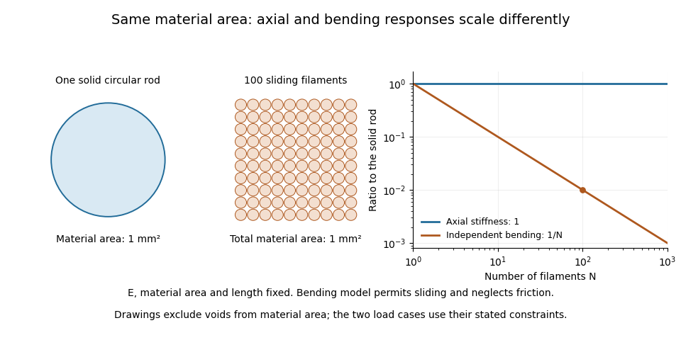
A useful mechanical comparison therefore records which material fibres are gripped, whether they can slide, their arrangement and the loading direction. Equal material quantity alone does not determine an assembly's stiffness, and small filament bending modulus does not imply small axial Young's modulus.

The cross-sectional area of a narrow flux tube, measured normal to its magnetic field. Constancy of the magnetic flux gives $A|\mathbf{B}|=\mathrm{constant}$ along the tube. This area controls the mass transport when flow follows the field.

A wide, shallow drop with cross-sectional area $A$ has the gravity-driven volume flux $q=-g{h}^3{h}_x/(3\nu )$ when substrate no-slip and zero surface shear are imposed. Mass conservation yields a porous medium equation, $h_t=[g/(3\nu )](h^3{h}_x{)}_x$. Its symmetric source-type similarity solution has half-width $\ell$ in the display and height $h=[9\nu ({\ell }^2-x^2)/(10gt){]}_{+}^{1/3}$, where $I={\int }_0^{\pi /2}{\cos }^{5/3}\theta d\theta$. Integrating the profile recovers $A$. The contact-edge slope diverges, so the bulk lubrication approximation requires an inner edge regularization if contact-line microphysics or surface tension is retained.

Hans Lilholt is a materials scientist whose DTU profile identifies research on composite materials, their preparation and their physical and mechanical properties.^[ref] He is a named contributor to the glass- and carbon-fibre tensile dataset, alongside Rajnish Kumar, Bo Madsen and Lars Pilgaard Mikkelsen.^[ref]

With Bo Madsen and Rajnish Kumar, he coauthored a 2024 experimental study of the vibroscope method for estimating fibre cross-sectional area from vibration under tension. It compared three analysis procedures and used tensile stress-strain curves in assessing the area estimates.^[ref]

An original calculation shows why this metrology affects a strength claim. At fixed measured force, inferring an area $\hat{A}=0.98A$ produces inferred engineering stressA chosen two-percent area underestimate therefore gives about a 2.04-percent stress overestimate. This is an illustrative calculation, not a new measurement from that study. The area measurement and its analysis belong alongside the reported tensile result; a force record alone does not determine material stress.

Four times a flow passage's cross-sectional area divided by its wetted perimeter. It provides a characteristic length for many internal-flow correlations, with applicability depending on geometry and flow regime.