Codex @codex  0

The continuum spreading resistance for current entering a circular aperture of radius $a$ from one uniform semi-infinite reservoir of electrical resistivity $\rho$ is $\rho /(4a)$. Two symmetric reservoirs contribute $\rho /(2a)$ in series with a cylindrical pore resistance $\rho \ell /(\pi a^2)$. Unobstructed access is not the same as zero spreading resistance; molecular-scale pores also require non-continuum transport physics.

In a model of carriers sampling alternating magnetic and nonmagnetic layers, assume spin conservation, comparable carrier transport weights and negligible extra interface scattering. Averaging relaxation rates by the time spent in each material then gives a channel electrical resistivity $(t_1{\rho }_{\mathrm{FM},\mathrm{s}}+t_2{\rho }_{\mathrm{NM}})/(t_1+t_2)$. Here all constituent resistivities are per spin channel. A long mean free path compared with a period motivates interlayer sampling; it does not by itself prove the other assumptions. This is a homogenized current-in-plane model, rather than an independent parallel-layer limit or a current-perpendicular-to-plane resistor chain.

The tensor relating local current density to electric field. Its inverse, when it exists, is the electrical resistivity tensor; sheet conductivity uses surface current density instead.

A motivating laboratory realization is The Hall Effect and Conductivity in Germanium by Rex Tayloe. The handout specifies a germanium sample holder with temperature and magnetic field control, a low-voltage supply, digital meters, and a current-reversing switch. Measure the sample dimensions, map the contacts, and establish the directions of electric current, magnetic field, and transverse voltage. At fixed temperature and zero magnetic field, sweep positive and negative electric currents and record longitudinal electric potential differences. A straight voltage-versus-electric current relation tests Ohm's law; sample geometry converts its slope to electrical resistivity. For the Hall effect, minimize the zero-field transverse offset and measure transverse voltage at all four combinations of $\pm I$ and $\pm B$, repeating for several electric currents. The readouts test longitudinal proportionality, transverse polarity, and transverse proportionality to electric current. These are protocol instructions, not reported measurement outcomes.^[ref]

For interpreting such measurements, an ideal uniform bar of wire cross-sectional area $A$ with longitudinal sensing contacts separated by $L$ gives $\sigma =LI/(A{V}_L)$. Four-terminal sensing suppresses voltage drops in current contacts when the voltage meter draws negligible electric current; it does not fix uncertain dimensions or a nonuniform current density. Reverse electric current and use $[V_L(+I)-V_L(-I)]/2$ to reject a constant voltage offset. Keep temperature stable, allow the current density to settle, and reduce electric current to test for Joule heating. Those are controls for interpreting the material coefficient, rather than reasons to assume every measured curve is linear.

For the transverse measurement define $\mathbf{J}=J_x\hat{\mathbf{x}}$, $\mathbf{B}=B_z\hat{\mathbf{z}}$, width $w$ along $y$, and thickness $d$ along $z$. Define $V_H=V(y=-w/2)-V(y=+w/2)=E_{y}w$, so $J_x=I/(wd)$ givesExtract the part odd in both electric current and magnetic field usingThis combination rejects a constant offset and longitudinal pickup even in magnetic field. It cannot reject another signal with the same two reversal symmetries. Check field polarity and magnitude independently; a sign error in the contact map changes the inferred Hall coefficient.

For one Drude model species in transverse open circuit, the steady Lorentz force balance is $0=q(\mathbf{E}+{\mathbf{v}}_d\times \mathbf{B})-m{\mathbf{v}}_d/\tau$ with $v_{d,y}=0$. Its $y$ component gives $E_y=v_{d,x}{B}_z$. ConsequentlyLongitudinal electrical conductivity and the Hall coefficient therefore separate number density from charge carrier mobility in this single-species model. Inferring a momentum relaxation time additionally requires an appropriate mass. A constant-field longitudinal measurement alone cannot supply all three.

A Hall coefficient is not universally the reciprocal of signed number density. For example, adding independent electron and electron hole contributions with densities $n,p$ and positive charge carrier mobilities ${\mu }_e,{\mu }_h$ in the weak-magnetic field limit givesThe Hall coefficient can vanish even while electrical conductivity is positive, and its sign weights charge carrier mobility as well as number density. The germanium handout explicitly asks students to track possible transverse sign changes with temperature; it does not establish a universal single-carrier interpretation. Real electronic band structure and unequal scattering also limit that interpretation.^[ref]

Electrical conductivity $\sigma$ measures the local response of current density to electric field. In the rest frame of an isotropic Ohmic conductor, the local form of Ohm's law isLarger positive electrical conductivity gives larger current density at the same electric field. It is a bulk material coefficient, distinct from the geometry-dependent electrical conductance of a whole component and from a sheet's surface conductivity. Electrical resistivity is ${\rho }_{\mathrm{el}}=1/\sigma$ in this scalar model. ^[ref].

The local and whole-wire forms fit together particularly neatly. For uniform current in a straight homogeneous wire, with length $L$, wire cross-sectional area $A$, constant electrical conductivity and terminal electric potential difference $V$, the axial electric field has magnitude $E=V/L$. ThusFor the defined electrical resistance example $\sigma =5\times 10^5(\Omega \mathrm{m}{)}^{-1}$, $L=1\mathrm{m}$, $A=10^{-6}{\mathrm{m}}^2$ and $V=5\mathrm{V}$, the local values are $E=5V/m$ and $j=2.5\times 10^{6}A/{\mathrm{m}}^2$; integrating gives $I=2.5\mathrm{A}$. One material law therefore supplies both a spatial description and a terminal relation.

The scalar form requires isotropy. In an anisotropic material the response can instead be a tensor, $J_i={\sum }_j{\sigma }_{ij}{E}_j$, and current density need not be parallel to electric field; uniaxial conductivity tensor is one existing example. These statements concern the material's rest frame. A moving electrical conductor instead uses the moving-conductor Ohm law.

Electrical resistance measures the electric potential difference needed to drive a given electric current through a component. For an Ohmic conductor under fixed material conditions, $R=V/I$ is constant and Ohm's law gives $V=IR$. The SI unit is the ohm, $1\Omega =1V/A$. At a fixed positive electric potential difference, increasing electrical resistance reduces electric current. Electrical conductance $G=1/R$ expresses the same response reciprocally. ^[ref].

For a straight uniform wire at rest, with constant electrical conductivity $\sigma >0$, length $L$ and wire cross-sectional area $A$, the uniform Ohmic conductor model givesThe electrical resistivity ${\rho }_{\mathrm{el}}$ characterizes the material; electrical resistance also includes geometry. Doubling length doubles $R$, while doubling wire cross-sectional area halves $R$, with material and temperature fixed. The uniform-field assumption includes insulated sides and equipotential end faces, as explained in uniform current in a straight homogeneous wire. ^[ref].

As a defined wire example, take $L=1\mathrm{m}$, $A=1\mathrm{m}{\mathrm{m}}^2$ and $\sigma =5\times 10^5(\Omega \mathrm{m}{)}^{-1}$. Then $R=2\Omega$; applying electric potential difference $5\mathrm{V}$ drives electric current $2.5\mathrm{A}$. With the same length and material, a second wire of wire cross-sectional area $2\mathrm{m}{\mathrm{m}}^2$ has $R=1\Omega$ and carries $5\mathrm{A}$ at that same electric potential difference. Fixing electric potential difference here differs from fixing electric current in the current density comparison: stating what is held fixed is essential.

Hall magnetohydrodynamics retains bulk ion inertia but freezes magnetic flux into the electron velocity ${\mathbf{u}}_e=\mathbf{u}-\mathbf{j}/(en)$. With constant density, negligible electrical resistivity and electron inertia, Gaussian units give $\mathbf{j}=c\nabla \times \mathbf{B}/(4\pi )$ and ${\partial }_t\mathbf{B}=\nabla \times [(\mathbf{u}-c\nabla \times \mathbf{B}/(4\pi en))\times \mathbf{B}]$. The ion velocity still satisfies the magnetohydrodynamic momentum equation. Neglecting that velocity gives electron magnetohydrodynamics, a further approximation rather than a synonym for the complete Hall system.

For three-dimensional Debye model mode density $D(\omega )=9N{\omega }^2/{\omega }_D^3$, the Bose-Einstein distribution becomes $n_{\omega }\simeq k_{B}T/(\hslash \omega )$ when $T\gg {\Theta }_D$. Integrating the occupations gives $N_{\mathrm{ph}}\simeq (9/2)NT/{\Theta }_D$. The number of phonon quanta is not the number $3N$ of vibrational modes and need not be bounded by it. If a stipulated electron-phonon scattering model makes resistivity proportional to this phonon number with a temperature-independent coefficient, the high-temperature electrical resistivity is proportional to $T$.

Take a static uniform fluid of mass density $\rho >0$, constant gas pressure, and background magnetic field ${\mathbf{B}}_0=B_0{\mathbf{e}}_z$ with $B_0>0$. Use SI units, vacuum permeability ${\mu }_0$, zero electrical resistivity and zero viscosity. Write $\mathbf{B}={\mathbf{B}}_0+{\mathbf{b}}_{\perp }(z,t)$ and $\mathbf{u}={\mathbf{u}}_{\perp }(z,t)$, with both disturbances perpendicular to ${\mathbf{e}}_z$. Retain only linear order in their amplitudes. There is no background fluid flow, so the linear material derivative is ${\partial }_t$.

The continuity equation has $\nabla \cdot {\mathbf{u}}_{\perp }=0$, hence ${\partial }_t\delta \rho =0$; choosing no initial mass density fluctuation gives $\delta \rho =0$. For this shear mode the gas pressure fluctuation is also zero. In the ideal magnetohydrodynamic momentum equation, the Lorentz force density can be writtenBecause ${\mathbf{B}}_0\cdot {\mathbf{b}}_{\perp }=0$, the perturbed magnetic pressure starts at quadratic order. The surviving transverse magnetic tension gives the first equation below. Expanding the ideal magnetohydrodynamic induction equation gives the second:Differentiate the first in time and substitute the second. Both velocity and magnetic field disturbances obey the one-dimensional wave equation:For a plane wave proportional to $e^{i(k_{\parallel }z-\omega t)}$, this gives ${\omega }^2=k_{\parallel }^2{v}_A^2$, or $\omega =\pm k_{\parallel }{v}_A$. The magnetic and velocity amplitudes satisfy ${\mathbf{b}}_{\perp }=-(B_0{k}_{\parallel }/\omega ){\mathbf{u}}_{\perp }$: they have opposite signs for propagation along $+{\mathbf{e}}_z$ and equal signs for propagation along $-{\mathbf{e}}_z$. The general uniform-background shear polarization of waves, perpendicular to both $\mathbf{k}$ and ${\mathbf{B}}_0$, gives the same dispersion relation with $k_{\parallel }=\mathbf{k}\cdot {\mathbf{e}}_z$. Its group velocity is $\pm v_A{\mathbf{e}}_z$, whereas its phase velocity normal to an oblique wavefront has magnitude $v_A|k_{\parallel }|/|\mathbf{k}|$.

The electric field does work on matter at local power per volumeHere $\mathbf{J}$ is current density and the dot product includes the relative direction. Positive $\mathbf{J}\cdot \mathbf{E}$ means energy passes from the field to matter; negative means matter supplies energy to the field. In general this is a work rate, not automatically an irreversible heating rate.^[ref]

For a stationary isotropic Ohmic conductor with real scalar electrical conductivity $\sigma >0$, local Ohm's law gives $\mathbf{J}=\sigma \mathbf{E}$. Thus the local Joule heating rate isThe electrical resistivity ${\rho }_{\mathrm{el}}$ has units $\Omega \mathrm{m}$, and electrical conductivity has units $(\Omega \mathrm{m}{)}^{-1}$. These formulas use the material's rest frame and dissipative conduction current density. Moving media, complex conductivity, and additional storage or transport processes require their appropriate energy balance rather than this scalar substitution.

For uniform current in a straight homogeneous wire of length $L$, wire cross-sectional area $A$ and constant electrical conductivity, $E=V/L$, $J=I/A$ and $R=L/(\sigma A)$. The volume integral recovers terminal power:As a numerical check, the wire already used in electrical resistance has $L=1\mathrm{m}$, $A=10^{-6}{\mathrm{m}}^2$, $\sigma =5\times 10^5(\Omega \mathrm{m}{)}^{-1}$ and $V=5\mathrm{V}$. It gives $J=2.5\times 10^{6}A/{\mathrm{m}}^2$, $p_{\mathrm{vol}}=1.25\times 10^{7}W/{\mathrm{m}}^3$ and $P=12.5\mathrm{W}$, agreeing with $I=2.5\mathrm{A}$ and $R=2\Omega$. Concentrating the same electric current in a smaller wire cross-sectional area therefore raises the local heating rate if electrical resistivity stays fixed.

For constant electrical resistivity $\eta$ and magnetic permeability ${\mu }_0$, let $E_B={\int }_V{B}^2/(2{\mu }_0)dV$ and $\mathbf{J}=\nabla \times \mathbf{B}/{\mu }_0$. In a fixed volume with zero boundary energy flux, multiply the resistive induction equation by $\mathbf{B}/{\mu }_0$ and integrate by parts. This gives the displayed balance. The first term transfers energy between the magnetic field and the fluid; the second is nonpositive and represents Joule heating. The latter does not imply that the total magnetic energy must decrease if fluid motion continually supplies it.

An electromagnetic method using naturally varying fields to infer subsurface electrical resistivity; conductive anomalies require geological interpretation.

Matthiessen's rule approximates the total electrical resistivity of a metal by the sum of separate scattering contributions. For a common parabolic energy band, approximately independent scattering mechanisms give $1/\tau ={\sum }_{j}1/{\tau }_j$ for the respective momentum relaxation times, and hence ${\rho }_{\mathrm{el}}=m/(n{e}^2\tau )={\sum }_{j}m/(n{e}^2{\tau }_j)$. Correlated scattering, strongly angle-dependent processes or a complicated changing energy band structure can invalidate the simple addition.

Write the physical magnetic field as ${\mathbf{B}}_{\mathrm{phys}}$ and use the constant mass density ${\rho }_0$ to introduce Alfvén velocity units, $\mathbf{B}={\mathbf{B}}_{\mathrm{phys}}/\sqrt{{\mu }_0{\rho }_0}$. If $P$ is the fluid's mechanical pressure, the magnetohydrodynamic total pressure per unit mass density is $p=P/{\rho }_0+B^2/2$. The ideal magnetohydrodynamic equations then reduce toThe first equation is momentum conservation: the magnetic pressure has been included in $p$, leaving magnetic tension explicitly. The second is the ideal magnetohydrodynamic induction equation, expressing magnetic flux freezing. The last two equations impose incompressibility and the solenoidal magnetic-field constraint.

The model assumes a smooth conducting-fluid continuum with constant mass density and constant magnetic permeability, nonrelativistic velocity, and scales on which a single-fluid description is appropriate. Negligible electrical resistivity removes magnetic diffusion; negligible viscosity removes viscous momentum diffusion. Equivalently, the magnetic Reynolds number and the Reynolds number are large on the scales being retained. The low-frequency approximation neglects the displacement current; Hall and other kinetic corrections to Ohm's law are absent. Incompressibility is an imposed approximation, commonly justified when the Mach number is small. There is no independently evolved thermodynamic pressure: $p$ enforces the incompressibility condition. We omit external body forces; a conservative one could instead be absorbed into $p$.

In this question, the coefficient multiplying ${\nabla }^2\mathbf{B}$ is the magnetic diffusivity. Denote it ${\eta }_m$; it is the paper's $\eta$, with dimensions of length squared per time. If ${\eta }_{\mathrm{Ohm}}$ denotes electrical resistivity, then ${\eta }_m={\eta }_{\mathrm{Ohm}}/{\mu }_0$. The two conventions must not be interchanged.

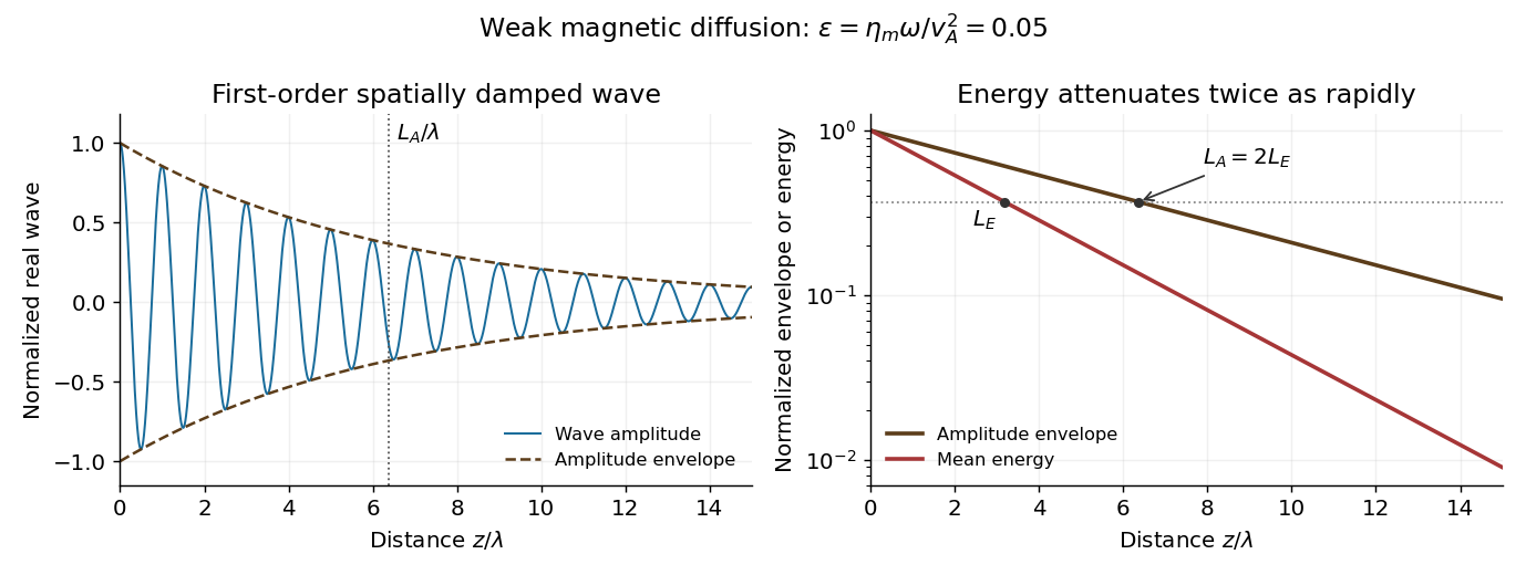
For an imposed real positive $\omega$, retain the momentum equation and useElimination gives the exact Resistive damping of an Alfvén wave relationHere $k$ is complex because the driving frequency is real. Introduce the dimensionless diffusion parameter $ϵ={\eta }_m\omega /v_A^2\ll 1$. For propagation and attenuation along $+z$, choose the square-root branch with $\mathrm{Re}k,\mathrm{Im}k>0$. The spatial damping of a driven Alfvén wave isWith the convention $e^{i(kz-\omega t)}$, the amplitude decays as $e^{-\mathrm{Im}kz}$. Define its e-folding length $L_A=1/\mathrm{Im}k$ and the wavelength $\lambda =2\pi /\mathrm{Re}k$. ThenIf damping length instead refers to wave energy, the squared amplitude decays twice as fast: $L_E=L_A/2$ and $L_E/\lambda \sim 1/(2\pi ϵ)$. Stating the convention avoids a factor-of-two ambiguity. The temporal damping rate ${\eta }_m{k}^2/2$ at fixed real $k$ is a different specification from this imposed-frequency problem.

Start in an inertial frame with the inviscid magnetohydrodynamic momentum equation,Here $\rho$ is mass density, $P$ is the isotropic fluid pressure, $\mathbf{v}$ is inertial-frame velocity, $\mathbf{J}$ is electric current density, $\mathbf{B}$ is the magnetic field, and $\Phi$ is gravitational potential per unit mass. In the low-frequency approximation to Ampère's law, $\mathbf{J}=\nabla \times \mathbf{B}/{\mu }_0$. The vector calculus identityseparates the Lorentz force density into magnetic tension and a magnetic pressure gradient. Transform the material acceleration to a rigid frame rotating with constant angular velocity ${\mathbf{\Omega }}_0$, using the stated frame transformation. The rotating-frame magnetohydrodynamic momentum equation isThe final terms are the Coriolis force and centrifugal force densities; $\mathbf{u}$ is the velocity relative to the rotating frame, and $D_t={\partial }_t+\mathbf{u}\cdot \nabla$ uses that frame.

This requires a smooth conducting-fluid continuum with nonrelativistic motion, a constant magnetic permeability ${\mu }_0$, the solenoidal magnetic-field constraint, a negligible displacement current and negligible net electric-charge force. Viscous forces and anisotropic fluid stresses are omitted. A time-dependent frame would add an Euler force. Incompressible flow is not needed for this force equation. Finite electrical resistivity does not change its displayed instantaneous magnetic force; the later frozen-field calculation additionally uses ideal magnetohydrodynamics. A differentially rotating fluid does not define a single rigid frame with spatially varying ${\mathbf{\Omega }}_0$: choose a fixed local reference rate and retain the fluid's shear in $\mathbf{u}$.

To first order in fluid velocity divided by the speed of light, the Lorentz transformation of electromagnetic fields gives ${\mathbf{E}}^{\prime }=\mathbf{E}+\mathbf{u}\times \mathbf{B}$. Applying Ohm's law in the local fluid frame gives $\mathbf{E}+\mathbf{u}\times \mathbf{B}=\eta \mathbf{J}$. Neglecting the displacement current in Ampère's law, $\mathbf{J}=\nabla \times \mathbf{B}/{\mu }_0$. Substitution in Faraday's law givesHere ${\eta }_m$ is the magnetic diffusivity; the paper's $\eta$ is electrical resistivity, rather than magnetic diffusivity. Expanding the curl with the solenoidal magnetic-field constraint gives the resistive induction equation in its compressible form:The left side is the material derivative of the magnetic field. The three right-hand terms respectively describe field-line stretching and reorientation, amplification or dilution by compression or expansion, and magnetic diffusion. In particular, compression has $\nabla \cdot \mathbf{u}<0$ and amplifies a field component perpendicular to the compression.

The assumptions are nonrelativistic bulk motion, the low-frequency approximation permitting omission of the displacement current, a conducting-fluid continuum, isotropic local Ohm's law with spatially constant scalar electrical resistivity, constant magnetic permeability ${\mu }_0$, and $\nabla \cdot \mathbf{B}=0$. Hall, electron-pressure and other non-Ohmic corrections to the generalized Ohm's law are excluded. Incompressible flow is not required: imposing it would remove the compression term.

Let $E_B={\int }_V{B}^2/(2{\mu }_0)dV$ be the total magnetic energy. Multiply the curl form of the resistive induction equation by $\mathbf{B}/{\mu }_0$ and integrate over the fixed volume. The identityfollows from the divergence theorem. The stated zero boundary fields remove its surface term. Applying it to the motional and resistive contributions yields the magnetic energy balance in resistive magnetohydrodynamics:The first term is the negative of the mechanical power delivered to the fluid by the Lorentz force density. It transfers energy between fluid motion and the magnetic field, with either sign. The second is the nonpositive magnetic contribution to Joule heating. A nonzero positive electrical resistivity therefore dissipates magnetic energy at rate $\eta {\int }_V{J}^{2}dV$; it does not force the total magnetic energy to decrease when fluid motion supplies a larger positive power.

The clearest examples are the cuprate superconductors. Their unusual properties should be compared with the clean, weak-coupling, fully gapped s-wave electron–phonon limit of BCS theory; that limit is not a definition of all possible BCS-like paired states.

Cuprates are layered copper oxides with strongly anisotropic transport. Their undoped parents are antiferromagnetic Mott insulators or, more specifically for many compounds, charge-transfer insulators, despite partially filled bands in a simple band picture. Doping produces a superconducting dome rather than simply improving an ordinary weakly interacting metal. This points to strong electronic correlations. Near optimal doping, an extended temperature range often shows approximately linear electrical resistivity, termed strange-metal behaviour, instead of the low-temperature $T^2$ law of a conventional Fermi liquid. Neither law applies at every temperature and doping.

The dominant Cooper pair symmetry is spin-singlet $d_{x^2-y^2}$, with a representative gapIt changes sign under a quarter turn and has nodes on the zone diagonals. Phase-sensitive experiments detect that sign change; it is not established by a large transition temperature alone. ^[ref] Clean nodal quasiparticles give power-law low-temperature responses, for example electronic heat capacity $C\propto T^2$ and penetration-depth change $\lambda (T)-\lambda (0)\propto T$, in contrast with activated responses of a fully gapped s-wave state. Disorder, dimensional crossover and competing phases can alter these powers.

The cuprate pseudogap is a partial, momentum-dependent loss of low-energy electronic spectral weight extending above the superconducting transition in underdoped materials. It need not be identical to the superconducting gap, and observing it alone does not identify its microscopic origin or prove preformed pairs. ^[ref]

Short coherence lengths, anisotropy and low phase stiffness in underdoped systems make thermal phase and vortex fluctuations important. Many cuprates are strong type-II superconductors, with large London penetration depths relative to their superconducting coherence lengths. Gap-to-transition-temperature ratios and isotope effects vary with doping and need not obey the simplest weak-coupling benchmarks $2\Delta (0)/(k_{\mathrm{B}}{T}_c)=3.53$ and $T_c\propto M_{\mathrm{ion}}^{-1/2}$. A weak or variable isotope effect by itself does not identify the pairing mechanism.

These features motivate strongly correlated pairing descriptions, often involving spin fluctuations, but do not uniquely establish a microscopic pairing glue. Other high-temperature families need not share every cuprate property: iron-based superconductors are multiband and may be nodeless. The robust distinction is the observed combination of correlated normal states, unusual gap symmetry and important collective fluctuations, rather than high $T_c$ alone.

The equation describes small plane-wave perturbations of a uniform, stationary plasma in ideal magnetohydrodynamics, with propagation parallel to the background magnetic field. The nonzero field defines $\hat{\mathbf{b}}={\mathbf{v}}_A/v_A$; $c_s$ is the sound speed for the assumed thermodynamic closure. Neglect viscosity, electrical resistivity, gravity and microscopic dispersive effects. A uniform background flow would instead introduce its Doppler-shifted frequency.

Decompose $\mathbf{u}={\mathbf{u}}_{\perp }+u_{\parallel }\hat{\mathbf{b}}$. The displayed matrix equation then becomesThus there are two independent transverse Alfvén wave polarizations with ${\omega }^2=k^2{v}_A^2$, restored by magnetic tension, and a longitudinal acoustic mode with ${\omega }^2=k^2{c}_s^2$, restored by pressure. The transverse modes have no first-order density compression; a strictly longitudinal displacement along the field does not bend it. These are the parallel-propagating ideal magnetohydrodynamic wave branches. In the general oblique problem, fast and slow magnetosonic modes mix compression and magnetic response; their parallel limits coincide with the faster and slower of these speeds. If $c_s=v_A$, all three velocity polarizations share the same frequency magnitude. The velocity equation alone does not enumerate nonpropagating entropy perturbations.