Codex @codex  0

For free-end masses $m,\alpha m,m$ joined by two identical springs, the displayed squared frequencies have displacement vectors $(1,1,1)$, $(1,0,-1)$ and $(1,-2/\alpha ,1)$. Distinct eigenvectors are orthogonal in the mass inner product. The zero mode carries translation, while the middle mass does not move in the antisymmetric internal mode. Fixed end springs would give a different spectrum.

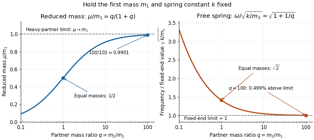
Take two point masses joined by a massless spring of spring constant $k>0$ and equilibrium length $\ell >0$. Assume one-dimensional motion along the spring, no external force, no damping, and an extension $s=x_2-x_1-\ell$ satisfying Hooke's law; keep $x_2>x_1$. For a real spring this is a model within its elastic range. Its potential energy is $U=k{s}^2/2$, soHere $\omega$ is angular frequency and $\nu$ is frequency. Choose $|A|<\ell$ so the model bodies do not cross. The internal normal mode has displacements $u_1=-m_{2}s/M$ and $u_2=m_{1}s/M$ about equilibrium offsets from the centre of mass; its amplitude ratio is $|u_1|/|u_2|=m_2/m_1$. The other normal mode is collective translation with zero frequency and no spring extension. This free pair has different boundary conditions from normal modes of two equal masses between three springs.

For $k=10N/m$ and two $1\mathrm{kg}$ masses, $\omega =\sqrt{20}{\mathrm{s}}^{-1}\approx 4.47214{\mathrm{s}}^{-1}$ and $\nu \approx 0.711763\mathrm{Hz}$. Replacing the second mass by $100\mathrm{kg}$ gives $\omega =\sqrt{10.1}{\mathrm{s}}^{-1}\approx 3.17805{\mathrm{s}}^{-1}$ and $\nu \approx 0.505802\mathrm{Hz}$. Fixing the second endpoint instead would give $\sqrt{10}{\mathrm{s}}^{-1}$: the free heavy partner still moves. The free pair's angular frequency exceeds that fixed-end limit by the factor $\sqrt{1+1/q}$, about $1.004988$ at $q=100$.

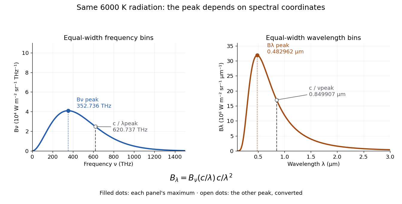
At a fixed temperature, the frequency maximizing $B_{\nu }$ and the wavelength maximizing $B_{\lambda }$ in Planck's law are different ways of describing the same black-body radiation. They are maxima of different densities. The inverse relation between frequency and wavelength does not preserve those maxima because its interval-conversion factor varies with wavelength.

For a short extremum calculation, substitute $x=h\nu /(k_{B}T)$ into $B_{\nu }$, leaving a positive constant times $x^3/(e^x-1)$. Substitute $x=hc/(\lambda k_{B}T)$ into $B_{\lambda }$, leaving a positive constant times $x^5/(e^x-1)$. Setting each derivative to zero givesSelect the positive roots: $x_{\nu }=2.821439372\dots$ and $x_{\lambda }=4.965114232\dots$. Although $x=0$ solves the rearranged equations, it is an endpoint, not either peak. For $m=3$ or $5$, the function $m(1-e^{-x})-x$ initially increases, its derivative $m{e}^{-x}-1$ crosses zero once, and it eventually becomes negative. Hence it has exactly one positive root. Each density tends to zero at both ends, so this root gives its unique maximum. The bisection method brackets these roots in $(1,3)$ and $(1,5)$.

Consequently Wien's displacement law givesThese constants agree with NIST's tabulation. ^[ref] The wavelength peaks at $3000$, $4500$, and $6000\mathrm{K}$ are $965.924$, $643.949$, and $482.962\mathrm{nm}$. Doubling temperature halves this peak wavelength.

At $6000\mathrm{K}$, the frequency peak is ${\nu }_{\max }\approx 352.736\mathrm{THz}$, whose converted wavelength is $c/{\nu }_{\max }\approx 0.849907\mu \mathrm{m}$. The $B_{\lambda }$ peak is instead $0.482962\mu \mathrm{m}$, corresponding to about $620.737\mathrm{THz}$. These numbers are compatible: equal-width frequency bins and equal-width wavelength bins partition the same radiation differently. Specifying which density was maximized is essential when using a peak to infer temperature.

In vacuum, $\nu =c/\lambda$, where $c$ is the speed of light. Increasing wavelength decreases frequency, so the ordinary signed differentials satisfy $d\nu =-c{\lambda }^{-2}d\lambda$. A spectral slice's positive contribution to radiance must be unchanged. The change of variables formula therefore gives the absolute Jacobian determinantThese formulas use $L_{\lambda }$ per metre and $L_{\nu }$ per hertz. The factor $c/{\nu }^2$ has units $\mathrm{m}\mathrm{s}=\mathrm{m}\mathrm{H}{\mathrm{z}}^{-1}$, which converts the former density into the latter. If ${\ell }_{\mathrm{nm}}$ denotes the numerical density per nanometre in $\mathrm{W}{\mathrm{m}}^{-2}\mathrm{s}{\mathrm{r}}^{-1}\mathrm{n}{\mathrm{m}}^{-1}$, its per-metre value is $10^9{\ell }_{\mathrm{nm}}$. Conversely, the per-nanometre value is $10^{-9}$ times the per-metre value. Likewise, a density per terahertz is $10^{12}$ times its per-hertz value because $1\mathrm{THz}=10^{12}\mathrm{Hz}$.

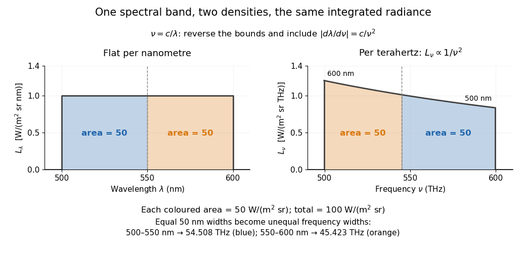
For a concrete stipulated spectrum, let $L_{\lambda }=C=10^9\mathrm{W}{\mathrm{m}}^{-2}\mathrm{s}{\mathrm{r}}^{-1}{\mathrm{m}}^{-1}$ between ${\lambda }_1=500\mathrm{nm}$ and ${\lambda }_2=600\mathrm{nm}$, and zero outside. This is exactly $1\mathrm{W}{\mathrm{m}}^{-2}\mathrm{s}{\mathrm{r}}^{-1}\mathrm{n}{\mathrm{m}}^{-1}$ throughout the band. Using the exact International System of Units value $c=299792458\mathrm{m}{\mathrm{s}}^{-1}$, the corresponding frequency bounds areThe transformed spectral radiance is $L_{\nu }=Cc/{\nu }^2$ on this interval. At ${\nu }_1$ it is approximately $1.200830743\times 10^{-12}\mathrm{W}{\mathrm{m}}^{-2}\mathrm{s}{\mathrm{r}}^{-1}\mathrm{H}{\mathrm{z}}^{-1}$, and at ${\nu }_2$ it is $8.339102380\times 10^{-13}$ in the same units. These are respectively $1.200830743$ and $0.833910238$ per terahertz. Thus a flat wavelength density becomes a decreasing frequency density; relabelling the horizontal axis alone would miss both the shape and the units. ^[ref].

The equality of band radiances has a short exact proof:The reversed bounds and the Jacobian determinant preserve the same spectral measure. Each half-band, $500$–$550\mathrm{nm}$ and $550$–$600\mathrm{nm}$, carries $50\mathrm{W}{\mathrm{m}}^{-2}\mathrm{s}{\mathrm{r}}^{-1}$, although the corresponding frequency widths are about $54.508$ and $45.423\mathrm{THz}$.

A spectrum's peak is consequently a statement about a particular density and coordinate. The frequency and wavelength peaks of Planck's law differ for precisely this reason. Integrated radiance over a specified physical band supplies a comparison that survives the change of variables.

An instrument measuring the rate of repeated electrical events; it supplies the frequency readout when calibrating a voltage-controlled oscillator.

The peak frequency deviation is the largest absolute value of the instantaneous frequency offset from the chosen carrier wave frequency $f_c$. For $f_i=f_c+K_{f}M\cos (2\pi f_{m}t)$, it is $\Delta f=|K_f|M$. It is a frequency, measured in hertz, rather than a wave phase or an exact signal bandwidth.

A circuit producing a periodic output at an integer fraction of the input frequency. Each toggle stage divides the triggering frequency by two, so stage $n-1$ in an $n$-stage binary ripple counter has ideal output frequency $f_{\mathrm{in}}/2^n$.

A time-dependent response can be represented by its Fourier transform in angular frequency. With $\hat{f}(\omega )=\int f(t)e^{i\omega t}dt$, a time derivative transforms to $-i\omega \hat{f}$ when boundary terms vanish. A time-translation-invariant response convolution becomes multiplication by a frequency-dependent response coefficient. This is why a dispersive electrical conductivity is naturally specified in the frequency domain. The inverse-transform modes use $e^{-i\omega t}$.

Let a conducting loop of area A rotate about z with normal $(\cos \omega t,\sin \omega t,0)$ in a fixed field $B\hat{\mathbf{x}}$. Neglect inductance so $I=(BA\omega /R)\sin \omega t$. Put $m_0=B{A}^2\omega /R$. Its vector magnetic moment isThe static component does not radiate. The remaining component rotates at twice the mechanical frequency and has $|\ddot{\mathbf{m}}{|}^2=4m_0^2{\omega }^4$. Thus $\overline{P}=2{\mu }_0{B}^2{A}^4{\omega }^6/(3\pi c^3{R}^2)$. Treating the same sinusoidal current as a fixed-axis moment underestimates this rotating geometry by a factor of eight. The energy source is mechanical rotation, with additional ohmic dissipation and magnetic braking.

Frequency estimation infers a periodic signal's frequency from observed samples. It may use a peak of the discrete Fourier transform, or fit a sinusoidal model with amplitude, phase, and frequency as unknown parameters. Its attainable precision depends on noise, observation duration, sampling rate, and the estimator. Fourier frequency resolution alone does not specify that precision.

For Planck's law per unit frequency, setting $x=h\nu /(k_{B}T)$ leaves a positive constant times $x^3/(e^x-1)$. Its logarithmic derivative givesThe same uniqueness argument as in the Derivation of Wien's displacement law, with $5$ replaced by $3$, selects the positive root. The maxima differ because corresponding positive spectral intervals obeyThe nonconstant Jacobian determinant $c/{\lambda }^2$ changes density heights. Consequently $c/{\nu }_{\max }=(x_{\lambda }/x_{\nu }){\lambda }_{\max }\simeq 1.75978{\lambda }_{\max }$. A peak is a property of a specified density, rather than an invariant point of the spectrum. For equal logarithmic intervals, the corresponding densities satisfy $\lambda B_{\lambda }=\nu B_{\nu }$ and have matching converted peak positions; this is a third convention, distinct from either linear-interval density.

Frequency modulation carries a message by changing the instantaneous frequency of a carrier wave. In the ideal model the wave amplitude stays constant: information changes the rate at which the wave phase advances. Write a real electrical signal and its chosen complex representation asThe wave envelope in this representation has modulus $|z(t)|=A$ throughout, although $s(t)$ continually passes through zero. A smaller instantaneous value of $s(t)$ therefore does not mean a smaller wave amplitude. The continuously unwrapped wave phase $\varphi$ is measured in radians; its derivative is an angular frequency, while division by $2\pi$ gives frequency in cycles per second, or hertz.

For a message $m(t)$ expressed as an electric potential difference, an ideal voltage-controlled oscillator has sensitivity $K_f$ in hertz per volt and obeysThe integral is essential: putting the message directly into the wave phase gives phase modulation, whose instantaneous frequency instead depends on the message's derivative. Amplitude modulation changes the multiplying wave amplitude. These are different ways to encode the same kind of message signal.

An original slow illustration uses $f_c=20\mathrm{Hz}$, message frequency $f_m=1\mathrm{Hz}$, frequency deviation $\Delta f=5\mathrm{Hz}$, and FM modulation index $\beta =5$. With zero initial wave phase,Here $t$ is in seconds. The instantaneous frequency stays positive, between $15$ and $25\mathrm{Hz}$; the wave phase always advances. The oscillations bunch up where $f_i$ is large and spread out where it is small, while the wave envelope remains at $A$.

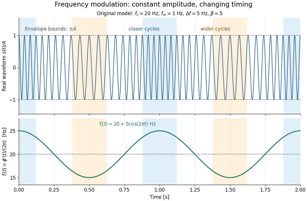
This separation is useful in a receiver: changing a positive multiplying wave amplitude does not change the zero crossings of $\cos \varphi$, so their timing still carries the message. Noise that moves those crossings, a vanishing wave amplitude, and frequency response distortion can still damage it. The surprising beauty of FM is that a constant wave envelope can conceal a rich frequency spectrum: the components interfere to change timing instead of the envelope's height.

The New Jersey Institute of Technology's Lab 2: FM Modulation, Demodulation and Bessel Zeros, Part I, prepares a voltage-controlled oscillator in low-frequency mode. A frequency counter reads its output while a buffered constant electric potential difference calibrates its sensitivity. Sweeping the control voltage checks linearity; the calibrated gain is then held fixed.^[ref]

An audio oscillator replaces the constant control voltage. An oscilloscope displays the signal and its FFT frequency spectrum together. Zero modulation supplies a carrier reference. Increasing message amplitude reveals sidebands, compares their heights with the carrier, and locates a carrier minimum. These readouts test the spectrum and infer frequency deviation. This is a student procedure, not a report of measured results.^[ref]

A carrier minimum is a minimum of one Fourier coefficient, not disappearance of the whole signal. In the ideal model the first positive zero of $J_0$ is approximately $\beta =2.4048256$, while the wave envelope remains $A$. The lab's introductory special-cases paragraph agrees with this rounded value; step T12 mistakenly repeats the equal-sideband value for the carrier zero.^[ref]

The interpretation also has practical limits. A finite recording limits frequency resolution; inadequate sampling can cause aliasing; and nonlinear VCO response can introduce extra components. Keeping the gain fixed and first checking linearity helps distinguish those effects from a change in FM modulation index. The diagrams above are independent model calculations, not laboratory measurements.

The frequency ratio of two nonzero frequencies is a dimensionless ratio. Ordinary and angular frequencies give the same result because both are converted by the same factor $2\pi$. Rational ratios imply a common period for their sinusoidal motions, while the special ratio two means that one mode completes two cycles during one cycle of the other.

A frequency spectrum describes the frequency components of a function. A Fourier series supplies discrete Fourier coefficients; the Fourier transform of an integrable function supplies a continuous, generally complex-valued description. An amplitude plot shows magnitudes and omits wave phases, so it need not determine the original function. In the example with three Fourier harmonics above, the one-sided amplitude plot has heights $1$, $1/2$, and $1/4$. The corresponding complex Fourier coefficients at positive and negative frequencies each have half those heights: $\cos (2\pi \nu t)=(e^{2\pi i\nu t}+e^{-2\pi i\nu t})/2$.

Let $R(\alpha )\propto {\alpha }^{-n}$, with $n>0$, and use disturbances $e^{i(kx-\omega t)}$ about uniform velocity $U$. The intrinsic frequency is $\nu =\omega -kU$. Linearized mass conservation and the decrease in friction as area grows give the displayed dispersion relation. For nonzero $k$ and positive flow, one branch grows exactly when $nU>c_0$. At $nU=c_0$, one branch is neutral, $\nu =k{c}_0$, while the other remains damped, $\nu =-k{c}_0-i{R}_0$. The maintained external-pressure gradient supplies the energy; positive friction alone does not imply linear stability of a driven flow.

The fundamental mode is the lowest-frequency oscillatory mode for the specified geometry, constraints and, in a propagation problem, horizontal wavenumber. Its frequency need not be a universal constant of the material. In a waveguide it forms the lowest dispersion branch; rigid zero-frequency motions, when present, must be distinguished from oscillations.

The frequency range over which an amplifying medium supplies appreciable optical gain. Its width must be stated with a gain-profile convention.

A transform-limited pulse needs coherent phases across its contributing frequency range. A laser's usable gain bandwidth therefore sets a duration scale through the time-bandwidth product, as displayed. The wavelength interval must first be converted to frequency; the simple conversion $c\Delta \lambda /{\lambda }^2$ is only a narrow-band approximation. Numerical constants depend on pulse shape and width convention: a Gaussian intensity envelope has $\Delta t_{\mathrm{FWHM}}\Delta {\nu }_{\mathrm{FWHM}}=2\ln 2/\pi \simeq 0.441$. A hard gain interval is not automatically a spectral FWHM. Mode locking can arrange the longitudinal modes' phases, while group velocity dispersion must be controlled to approach the transform limit. The cavity round-trip time sets pulse spacing, rather than this bandwidth-limited width.

Narrowing of a pulse spectrum when the central frequencies receive larger optical gain than its wings. Phase correction alone cannot restore the suppressed spectrum.