Green's function

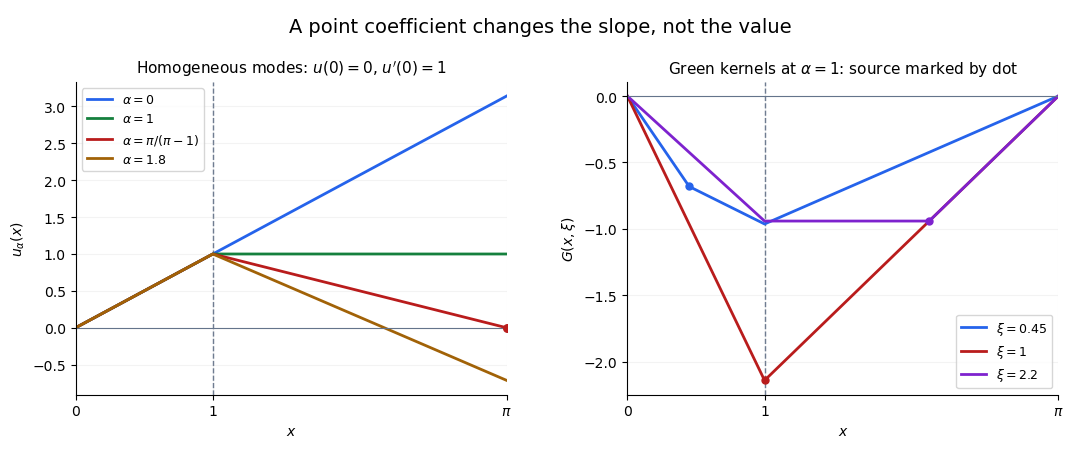
Multiplying the equation for $v=y^{\prime }$ by the integrating factor $e^x$ gives $v(x)=-e^{-x}{\int }_x^1{e}^{t}f(t)dt$. Integrating once more and reversing the order of integration gives the Green's functionIt is continuous across $x=t$, its first derivative has jump $+1$, and it satisfies the mixed Dirichlet boundary condition and Neumann boundary condition. Both homogeneous solutions, $1$ and $e^{-x}$, are eliminated by these two conditions, giving uniqueness. For $f=e^{-x}$ the solution is $-x{e}^{-x}$.

A continuous forcing gives the solution with zero initial data $z(x)=-{\int }_0^x\sin (x-s)f(s)ds$. Every solution vanishing at zero is $A\sin x+z(x)$. If $\sin L\ne 0$, the remaining endpoint determines $A$ uniquely, with Green's functionIts first derivative has jump $-1$, the correct sign for $-y^{\prime \prime }-y=f$. If $L=m\pi$ with a positive integer $m$, solvability instead requires ${\int }_0^{L}f(s)\sin sds=0$, and the coefficient $A$ is free. This is the Fredholm alternative with a one-dimensional homogeneous kernel.

variation of parameters with the fundamental solutions $x,x^2$ givesThe kernel is continuous across $x=t$ and its first derivative jumps by $t^{-2}$, which gives unit in a ring source after multiplication by the leading coefficient. It satisfies both endpoint conditions. The homogeneous solution $Ax+B{x}^2$ satisfies them only when $A=B=0$, proving uniqueness.

An adjoint Green's function solves the corresponding adjoint point-source problem, with boundary or terminal conditions chosen so that integration by parts gives a representation for a solution of the original operator. For $L={\partial }_t-{\partial }_x^2+c$ on the real line, the formal adjoint is $L^{\ast }=-{\partial }_t-{\partial }_x^2+c$. The backward kernel with terminal Dirac delta at $(\xi ,\tau )$ is the translated heat kernel with constant absorption, defined for $t<\tau$. Its pairing with a homogeneous forward solution is constant in $t$; taking the terminal limit evaluates that solution at $(\xi ,\tau )$.

For $L=a_2(x)D^2+a_1(x)D+a_0(x)$ with $a_2(\xi )\ne 0$, a Green's function solving $L_{x}G=\delta (x-\xi )$ is homogeneous on either side of $\xi$, continuous there, and has first derivative jump $[G_x{]}_{-}^{+}=1/a_2(\xi )$. A nonzero jump in $G$ itself would produce an unwanted distributional derivative of the Dirac delta. Once continuity removes that term, integrating the equation across $\xi$ fixes the derivative jump. Endpoint boundary conditions complete the classical characterization.

Suppose a linear ordinary differential operator satisfies $L(qv)=rMv$ on an interval, where the functions $q,r$ never vanish and homogeneous endpoint boundary conditions for $y=qv$ correspond to those used for $v$. If $G_M$ is a Green's function for $M$, then $Ly=f$ is equivalent to $Mv=f/r$, soThus the displayed kernel is the Green's function for the original, possibly non-normalized operator. The source factor belongs at $s$, while the dependent-variable factor belongs at $x$.

For $Ly=x^2{y}^{\prime \prime }-2x{y}^{\prime }+(x^2+2)y$ on $[\pi /2,\pi ]$ with zero endpoint values, $q=x$ and $r=x^3$ reduce the equation to $Mv=v^{\prime \prime }+v$. The kernel of $M$ is $\cos (x_{<})\sin (x_{>})$, where $x_{<}=\min (x,s)$ and $x_{>}=\max (x,s)$. Therefore $G_L(x,s)=x\cos (x_{<})\sin (x_{>})/s^3$. Its first derivative has jump $1/s^2$, as required by the leading coefficient $s^2$ of $L$.

For the quadrant $x,y>0$, the displayed Green function satisfies $\Delta G={\delta }_{(\xi ,\eta )}$, zero value on $y=0$ and zero outward normal derivative on $x=0$. The method of images uses the logarithmic fundamental solution of the Laplace equation with coefficient $1/(2\pi )$: keep the source sign when reflecting across the Neumann side and reverse it when reflecting across the Dirichlet side. The four image signs are therefore $+,+,-,-$ for sources $(\xi ,\eta ),(-\xi ,\eta ),(\xi ,-\eta ),(-\xi ,-\eta )$.

On $y=0$, equal numerator and denominator give zero. Evenness in $x$ gives the Neumann condition at $x=0$. The outward normal derivative on the Dirichlet side is the positive kernelGreen's second identity consequently gives $u(P)={\int }_{D}Gf+{\int }_{y=0}g{\partial }_{n}G$ for $\Delta u=f$ with these mixed boundary data, assuming any remote-boundary contribution vanishes. The sign convention is $\Delta G=+\delta$; changing to $-\Delta G=\delta$ changes both the Green function and the representation signs.

Let $h_1,\dots ,h_n$ be a basis of homogeneous solutions of a linear ordinary differential operator $L$ of order $n$. Let $B_1,\dots ,B_n$ be independent homogeneous linear boundary conditions, which may be coupled. Suppose a fundamental solution $G_0(x,\xi )$ satisfies $L_x{G}_0=\delta (x-\xi )$. Define the boundary matrix $M_{ij}=B_i{h}_j$ and $b_i(\xi )=B_i{G}_0(\cdot ,\xi )$. If $M$ is invertible, thenThe added terms are homogeneous solutions, so the Dirac delta source is preserved. Applying the boundary operators gives $b-M{M}^{-1}b=0$. Any two such Green functions differ, for fixed source position, by a homogeneous solution with coefficient vector in the null space of $M$; invertibility therefore proves uniqueness. A singular boundary matrix signals a nontrivial homogeneous solution satisfying the endpoint conditions, where a compatibility condition and a nonunique inverse may arise. For $L=D^2$, one convenient fundamental solution is $(x-\xi )H(x-\xi )$.

For the inverse transform $G(\tau )=\int d\omega e^{-i\omega \tau }g(\omega )/(2\pi )$, positive $\tau$ requires closing a decaying contour below the real axis, clockwise; negative $\tau$ requires closing above, counterclockwise. Poles strictly below give a retarded Green function, while poles strictly above give an advanced Green function. Real-axis poles need a prescription. The sign convention in the Fourier exponential is essential.

A static background permits a Fourier transform of time difference, but a spatially varying coefficient generally prevents dependence on position difference alone. A momentum-space Green function then carries an incoming and an outgoing momentum, or equivalently one momentum together with the source position. Multiplication by a background field becomes a convolution, with a source-position phase when the Fourier basis is written as $e^{i\mathbf{k}\cdot (\mathbf{r}-{\mathbf{r}}^{\prime })}$. A diagonal single-momentum representation is justified only with additional spatial translation symmetry or an explicitly fixed source origin.

An advanced Green function has support only before its source time. It is selected by a future boundary condition, rather than an initial causal response. For $L={\partial }_t^2+2\lambda {\partial }_t+{\omega }_0^2$ with $\lambda <0$ and ${\Omega }^2={\omega }_0^2-{\lambda }^2>0$, the real-axis inverse Fourier transform of $(-{\omega }^2-2i\lambda \omega +{\omega }_0^2{)}^{-1}$ is $-H(-t)e^{-\lambda t}\sin (\Omega t)/\Omega$. Its first derivative jumps by one at zero. A growing retarded solution exists with a different inverse contour; this illustrates causality versus stability of a Green function.

A static but spatially inhomogeneous linear operator has time translation symmetry without spatial translation symmetry. At fixed source position ${\mathbf{r}}^{\prime }$, one may still Fourier transform its Green function in $\mathbf{x}=\mathbf{r}-{\mathbf{r}}^{\prime }$. The coefficient retains ${\mathbf{r}}^{\prime }$ as a parameter. A multiplication by $V(\mathbf{r})$ becomes a convolution with $V_{{\mathbf{r}}^{\prime }}(\mathbf{q})=e^{i\mathbf{q}\cdot {\mathbf{r}}^{\prime }}\tilde{V}(\mathbf{q})$, not a spatially diagonal multiplier unless $V$ is constant. Suppressing the source-position subscript is only a notational convention.

For a smooth bounded connected domain $V$ with boundary $S$, integrating the Green function equation and applying the divergence theorem forces ${\int }_S{\partial }_{n}GdS=1$. Thus zero Neumann boundary data are incompatible with an unmodified unit point source. The displayed constant boundary derivative has the required total flux. For $\Delta \Phi =\sigma$ and ${\partial }_n\Phi =f$, the compatibility condition is ${\int }_V\sigma dV={\int }_{S}fdS$. Green's second identity then yieldsThe last term is an undetermined additive constant. Adding a constant to $G$ does not change the other two terms together, because of the compatibility condition. This construction keeps the unit Dirac delta source; using a mean-subtracted source with zero normal derivative is a different normalization.

For $Ly=y^{\prime \prime }+y^{\prime }/x-y/x^2$ on $x>0$, impose $y(0)=0$ by a continuous limit and $y(x)\to 0$ at infinity. The adapted homogeneous solutions are $x$ at zero and $1/x$ at infinity, with Wronskian $-2/x$. The displayed Green function is continuous and its first derivative has jump one at $x=s$, so $L_{x}G(x,s)=\delta (x-s)$ with ordinary source measure $ds$. For continuous $f$ with ${\int }_0^{\infty }(1+s^2)|f(s)|ds<\infty$,This solves $Ly=f$ with the stated endpoint limits. No nonzero combination of $x,1/x$ meets both homogeneous endpoint conditions, proving uniqueness. Multiplying $L$ by $x$ gives the self-adjoint expression $(x{y}^{\prime }{)}^{\prime }-y/x$, explaining the weighted reciprocity $xG(x,s)=sG(s,x)$.

For $Ly=(x^2{y}^{\prime }{)}^{\prime }-2y$ on $x>0$, choose solutions bounded at zero and infinity. The homogeneous Cauchy-Euler equation has basis $x,x^{-2}$. Joining the left-regular and right-regular solutions continuously and imposing $s^2[G_x{]}_{s^{-}}^{s^{+}}=1$ gives the displayed Green's function with ordinary integration measure $ds$. For bounded forcing,The integrals converge and give the unique bounded solution: no nonzero homogeneous combination is bounded at both ends. If $0\le f\le M$, negativity of the kernel gives $-M/2\le y\le 0$. Differentiation cancels the two moving-endpoint terms, leavingwhich implies $|y^{\prime }(x)|\le M/(3x)$. For constant forcing $f=M$, the bounded solution is $-M/2$; the endpoint conditions are boundedness, rather than zero endpoint values.

For zero initial value and slope, the causal Green function is $G_0(x,s)=H(x-s)\sin [k(x-s)]/k$, with $k\ne 0$ and $H$ the Heaviside step function. For zero values at endpoints $a<b$, put $\kappa =|k|$. The Dirichlet Green function isBoth are continuous at the source and have a first-derivative jump of one, giving $L_{x}G=\delta (x-s)$. The Dirichlet inverse exists when $\sin [\kappa (b-a)]\ne 0$; a zero denominator signals a nontrivial homogeneous mode and a Fredholm solvability condition. The endpoint kernel is the zero-conjugation case of the Dirichlet Green function for a conjugated harmonic oscillator. Boundary conditions determine which kernel must be integrated against a forcing term.

The homogeneous Cauchy-Euler equation $Ly=0$ has fundamental solutions $x,x^{-1}$ on $x>0$, with Wronskian $-2/x$. Requiring decay at both endpoints gives the unweighted Green's functionRequiring zero initial value and derivative at zero instead gives the forward kernelBoth kernels are continuous and have first-derivative jump one at $x=\xi$, so $L_{x}G=\delta (x-\xi )$. Away from that point they solve the homogeneous equation. Integrating against the forcing with ordinary measure $d\xi$ yields the respective solutions whenever the integral and endpoint limits converge. Their difference is $G_0-G_D=x/2$, independent of $\xi$, so the solutions differ by the homogeneous term $(x/2)\int f(\xi )d\xi$ for integrable forcing. For example, the two choices for an indicator forcing on $(0,1)$ differ by $x/2$. Specifying a differential operator without its endpoint conditions does not specify its Green kernel.

For $0<x<1$, the homogeneous Cauchy-Euler equation has solutions $x,x^{-1}$. The left-vanishing solution $x$ and right-vanishing solution $x-x^{-1}$ give the unweighted Green function $G(x,s)=x(1-s^{-2})/2$ for $x\le s$ and $(x-x^{-1})/2$ for $x\ge s$. It is continuous at $x=s$ and its first derivative has jump $1/s^2$, so $L_{x}G=\delta (x-s)$.

For continuous forcing $f$ on $[0,1]$, its integral isThis is bounded at zero and vanishes at one, but $u(0^{+})=-f(0)$. The first singular term uses the average $x^{-1}{\int }_0^{x}f\to f(0)$. In the other, the substitution $t=x/s$ gives $x{\int }_x^{1}f(s)s^{-2}ds={\int }_x^{1}f(x/t)dt\to f(0)$ by dominated convergence. Thus the two zero endpoint values require $f(0)=0$. When compatible, the solution is unique among bounded solutions because no nonzero combination of $x,x^{-1}$ meets both homogeneous endpoint conditions. This example shows why pointwise endpoint behavior of a Green function does not itself justify passing a limit through its integral.

For $Ly=-x^{-2}(x^2{y}^{\prime }{)}^{\prime }+y$ on $x>0$, require boundedness at zero and at infinity. The substitution $z=xy$ reduces the homogeneous equation to $-z^{\prime \prime }+z=0$. The adapted solutions are $\sinh x/x$ at zero and $e^{-x}/x$ at infinity, with Wronskian $-x^{-2}$. The displayed Green function is continuous and has first-derivative jump $-1$, so $L_{x}G=\delta (x-\xi )$ with ordinary source measure $d\xi$. It satisfies weighted reciprocity $x^{2}G(x,\xi )={\xi }^{2}G(\xi ,x)$. For forcing equal to one on $[0,R]$ and zero outside, integration gives $y=1-(R+1)e^{-R}\sinh x/x$ inside and $y=(R\cosh R-\sinh R)e^{-x}/x$ outside. Limits define the regular value at zero.

The usual Green function formula for a monic second-order equation requires a nonzero Wronskian at the source. At an interior singular point it may fail to define an ordinary inverse for arbitrary forcing. For example, for $Ly=y^{\prime \prime }-(1+x)y^{\prime }/x+y/x$ on $[-1,1]$, choose $u=1+x$ and $v=e^x-e(1+x)/2$. They satisfy the left and right Dirichlet boundary conditions, and $W=u{v}^{\prime }-u^{\prime }v=x{e}^x$. The displayed kernel is valid for $\xi \ne 0$ and has unit jump in its first $x$ derivative. Its $1/\xi$ behaviour prevents unrestricted integration through zero. For smooth forcing $f(x)=xq(x)$, the product $G(x,\xi )f(\xi )$ has a removable singularity, and its integral gives the unique solution extending with two continuous derivatives through zero. That matching condition matters: merely requiring one continuous derivative allows additional piecewise homogeneous solutions. A smooth forcing with $f(0)\ne 0$ cannot have a solution with two continuous derivatives there, as expansion of $x{y}^{\prime \prime }-(1+x)y^{\prime }+y=xf$ shows.

Let $p(D)$ be a constant-coefficient differential operator, $D=d/dt$, with distinct characteristic roots ${\lambda }_j$ having nonzero real parts. The solution of $p(D)K=\delta$ decaying at both temporal infinities iswhere $H$ is the Heaviside step function. This follows by partial fraction decomposition of $1/p(z)$ and the first-order kernels $e^{\lambda t}H(t)$ for $\mathrm{Re}\lambda <0$, or $-e^{\lambda t}H(-t)$ for $\mathrm{Re}\lambda >0$. Both first-order kernels jump by one and solve $(D-\lambda )K_{\lambda }=\delta$ as distributions.

For example, $p(D)=(D+1)(D-2)(D+2)$ givesIt is continuous together with its first derivative; its second derivative jumps by one, as required by the jump conditions for a third-order Green function. A solution of $p(D)y=f$ is the convolution $K\ast f$ when it exists. If positive-real-part roots occur, decay at both ends generally requires a nonzero negative-time branch: this is the distinction captured by causality versus stability of a Green function. A causal kernel would retain growing positive-time terms and need not have a real-axis Fourier transform.

On $0<x<1$, both independent homogeneous solutions $x,x^3$ vanish at the singular endpoint zero. Consequently imposing $y(0)=y(1)=0$ leaves the nonzero homogeneous solution $x^3-x$ and does not determine a unique inverse. One valid right Green function, with $L_{x}G=\delta (x-z)$ and zero endpoint values, isIts first derivative has jump one because the Wronskian of $x$ and $x^3-x$ is $2z^3$. Every kernel $G_0+(x^3-x)h(z)$ preserves these properties when the integrals exist. For sources supported away from zero, integration yields one particular solution; the full endpoint-constrained family adds $C(x^3-x)$. An additional endpoint selection, such as $y(x)/x\to 0$, can choose a unique member. This is a singular-endpoint phenomenon, not an ordinary regular two-point uniqueness theorem.

For $0<a<b$, the displayed decaying Green function solves $(-{\partial }_x^2+a^2)(-{\partial }_x^2+b^2)K={\delta }_0$ on the real line. Its Fourier transform isInvert each term using the one-dimensional modified Helmholtz Green function. Then a decaying solution with forcing $h$ is the convolution $K\ast h$. For $a=1,b=2$, this gives $K=e^{-|x|}/6-e^{-2|x|}/12$ for the operator ${\partial }_x^4-5{\partial }_x^2+4$. Its first-derivative jump cancels, while its third-derivative jump is one, providing the unit Dirac delta distribution required by the fourth-order operator.

For $L=y^{\prime \prime }+\alpha y^{\prime }/x+(\alpha -1{)}^{2}y/(4x^2)$ on $x>0$, the repeated indicial root is $r=(1-\alpha )/2$ and the homogeneous solutions are $x^r,x^r\log x$. Their Wronskian is $x^{-\alpha }$. The displayed causal Green function is continuous at each source $\xi >0$, has a unit jump in its first derivative, and satisfies $L_{x}G=\delta (x-\xi )$. It is zero near the origin, so its value and first derivative there vanish. Those origin conditions alone fail to give uniqueness when $\alpha <-1$: then both homogeneous solutions and their first derivatives vanish as $x\downarrow 0$. For forcing $f(x)=x$, source integration from zero converges when $\alpha >-5$ and gives $y_p=4x^3/(\alpha +5{)}^2$. All zero-origin-data solutions in $-5<\alpha <-1$ are $y_p+x^r(C_1+C_2\log x)$; for $\alpha \ge -1$ the solution is unique. Causality selects the displayed kernel even when the bare singular-endpoint conditions are insufficient.

For $L=d^2/d{x}^2-2/x^2$ on $x>0$, the homogeneous solutions $x^2,x^{-1}$ satisfy respectively the zero and infinity boundary conditions. Their Wronskian is $-3$. The displayed Green's function is continuous at $x=\xi$ and its first derivative has jump one, so $L_{x}G=\delta (x-\xi )$ in the distribution sense. Integration against a compactly supported forcing gives the unique solution decaying at both boundaries.

For $L=d^2/d{x}^2+(2/x)d/dx+k^2$ on $0<x<1$, impose finiteness at zero and zero value at one. Set $H=xG$; then $H^{\prime \prime }+k^{2}H=\xi \delta (x-\xi )$ with ordinary zero-endpoint conditions. The displayed Green function follows from the left/right sine solutions, where $x_{<}=\min (x,\xi )$ and $x_{>}=\max (x,\xi )$. Its derivative jumps by one. It exists for $k\notin \pi \mathbb{Z}\setminus \{0\}$; at zero take the removable limit $G=-\xi x_{<}(1-x_{>})/x$. At nonzero integer multiples of pi the radial problem has a nonzero homogeneous solution and a Fredholm solvability condition. Integrating against the constant forcing gives $y=k^{-2}[1-\sin (kx)/(x\sin k)]$, with $y=(x^2-1)/6$ at $k=0$.

For the three-dimensional reference Green function $g(r)=1/(4\pi br)$, the distributional mixed Hessian $K={\nabla }_x{\nabla }_{x^{\prime }}g$ has the displayed contact and principal-value parts. Since the spherical mean of $n\otimes n$ is $I/3$, its ordinary dipole part has zero angular integral. Radial weighting therefore isolates the contact term, provided boundary truncation is absent or negligible in the bulk limit.

For a monic second-order operator, choose a homogeneous solution $u$ satisfying the left Robin boundary condition and a solution $v$ satisfying the right decay condition. With $W=u{v}^{\prime }-u^{\prime }v\ne 0$, the displayed kernel is continuous and its first derivative has jump one. It therefore satisfies $LG=\delta$ and the two boundary conditions. The operator's first derivative term generally makes $W$ nonconstant and the resulting Green function nonsymmetric in the unweighted variables.

With the positive logarithmic convention, a Green function with pole $p$ on a noncompact Riemann surface is positive and harmonic away from $p$, has local form $-\log |\zeta |$ plus a harmonic function in a coordinate $\zeta (p)=0$, and is minimal among positive functions with these properties. It is obtained, when finite, as the increasing limit of zero-boundary Green functions on an exhaustion by compact bordered subdomains. On the unit disk it isIts sign convention is $-\Delta G=2\pi {\delta }_p$ in a conformal coordinate, with the opposite overall sign from conventions using $\log |\zeta |$ as the singular part.

The impulse response records the response to a unit impulse, with specified initial or boundary conditions. In continuous time the impulse is a Dirac delta function; in discrete time it is the Kronecker delta $\delta [n]$. For a linear time-invariant system with zero initial state, the response to a general input is its convolution with the impulse response. The impulse response of a causal filter is zero before the impulse.

For the five-sample moving average, a discrete impulse produces $h[n]=1/5$ at $n=0,1,2,3,4$ and zero otherwise. The response lasts five samples, so this is a finite impulse response system. Its frequency response is the finite sum of the five delayed phase contributions: one short input experiment determines how every sustained sinusoid is filtered.

For $L_k=k{\partial }_z+k^{-1}{\partial }_{\bar{z}}$, $k\ne 0$, $|k|\ne 1$, this kernel satisfies $L_k{G}_k={\delta }_0$. A real-linear change of complex coordinate reduces its derivation to the Cauchy-Green operator; the determinant changes sign at the unit circle. For $|k|=1$ the operator becomes a real directional transport equation, whose characteristic singularity requires limiting prescriptions. The kernel has $G_k\sim k/(\pi z)$ at zero and $G_k\sim 1/(\pi k\bar{z})$ at infinity.

A Dirichlet Green function for a differential operator satisfies homogeneous Dirichlet boundary conditions in one variable. It converts source and boundary data into an integral representation of the solution.

For $L=-d^2/d{x}^2+1$ on $[-1,1]$ with zero endpoint values, the displayed Green kernel is positive and symmetric. Each side solves the homogeneous equation; the kernel is continuous at $x=s$ and its first derivative has jump $-1$. Hence $LG(\cdot ,s)={\delta }_s$. Integrating against a forcing function solves $Ly=f$. For the indicator of the right half-interval, the value at zero is $(\cosh 1-1)/(2\cosh 1)$, obtained by integrating $\sinh 1\sinh (1-s)/\sinh 2$ over $0\le s\le 1$. The derivative-jump sign changes if the operator is written with the opposite overall sign.

For $0<x<1$, consider the self-adjoint differential operator $L=(pd/dx{)}^{\prime }+q$ with $p=e^{-x}/(1-x)$ and $q=-e^{-x}/(1-x{)}^2$. The homogeneous solutions $u=x$ and $v=e^x-ex$ satisfy the left and right zero Dirichlet boundary conditions. Their Wronskian is $(x-1)e^x$, and $pW=-1$. Thus the displayed Dirichlet Green function is continuous, zero at both endpoints, and has unit flux jump $p(s)[G_x(s^{+},s)-G_x(s^{-},s)]=1$.

The right solution has a double zero, $v(s)\sim e(1-s{)}^2/2$. Consequently $G(x,s)F(s)$ is integrable at $s=1$ for fixed interior $x$ when $F(s)=-e^{-s}/(1-s{)}^2$, even though $F$ itself is not integrable there. The endpoint zero of the Wronskian causes no loss of this construction because the weighted Wronskian $pW$ stays nonzero. This illustrates the need to retain the integrating factor when constructing a Green function at a singular endpoint.

For the point interaction in a second-order differential equation $L_{\alpha }={\partial }_x^2+\alpha {\delta }_c$ on $(0,\ell )$, use homogeneous Dirichlet boundary conditions. The unperturbed Green function iswith a positive unit derivative jump at $x=\xi$. Whenever $1+\alpha G_0(c,c)\ne 0$,To derive this rank-one operator correction, move the delta coefficient to the right-hand side and apply the unperturbed inverse: $G_{\alpha }(x,\xi )=G_0(x,\xi )-\alpha G_0(x,c)G_{\alpha }(c,\xi )$. Setting $x=c$ determines $G_{\alpha }(c,\xi )$ and gives the formula. Its denominator vanishes exactly at Dirichlet resonance for a point interaction.

The kernel is symmetric. It is continuous at $x=c$ and $x=\xi$, satisfies $[{\partial }_x{G}_{\alpha }{]}_{\xi }=1$ when $\xi \ne c$, and satisfies $[{\partial }_x{G}_{\alpha }{]}_c=-\alpha G_{\alpha }(c,\xi )$ away from the source. When $\xi =c$, the single combined condition is $[{\partial }_x{G}_{\alpha }{]}_c=1-\alpha G_{\alpha }(c,c)$. These are the transmission conditions for a delta coefficient, including a source at the interaction.

For the gap $a<r<b$, put $u_{\ell }(r)=r^{\ell }-a^{2\ell +1}{r}^{-\ell -1}$, $v_{\ell }(r)=r^{-\ell -1}-r^{\ell }/b^{2\ell +1}$ and $d_{\ell }=(2\ell +1)[1-(a/b{)}^{2\ell +1}]$. With orthonormal spherical harmonics, the Dirichlet Green function isFor a short verification, $u_{\ell }(a)=v_{\ell }(b)=0$ and both solve the radial Laplace equation. Their Wronskian is $u_{\ell }{v}_{\ell }^{\prime }-u_{\ell }^{\prime }{v}_{\ell }=-d_{\ell }/r^2$. Thus the radial derivative jump is $-1/r^{\prime 2}$; completeness of the spherical harmonics gives the stated Dirac delta function normalization. A point charge has electric potential $qG/(4\pi {ϵ}_0)$, and the inner-wall surface charge density is $-q{\partial }_{r}G{|}_{a^{+}}/(4\pi )$, with the angular source coordinates held fixed.

For $D=\{x>0,z>0\}\subset {\mathbb{R}}^3$, take the Dirichlet Green function convention $-{\Delta }_{P}G(P,Q)={\delta }_Q(P)$. Reflect $Q=(\xi ,\eta ,\zeta )$ to $Q_{ij}=((-1{)}^i\xi ,\eta ,(-1{)}^j\zeta )$. The displayed image sum vanishes on both faces, has exactly one positive unit source inside $D$, and decays at infinity. Pairwise cancellation proves the boundary conditions, while the three image terms are harmonic inside $D$. Its inward source-normal derivative gives the Poisson kernel of a three-dimensional quarter-space. The source sign must be kept consistent with Green's second identity.

For the face $z=0$ of $x>0,z>0$, set $r_{\mp }^2=(x\mp \xi {)}^2+(y-\eta {)}^2+z^2$, with source boundary coordinates $\xi >0$, $\eta \in \mathbb{R}$. The Poisson kernel for data on that face and zero data on $x=0$ is the displayed positive difference. It follows by differentiating the Dirichlet Green function for a three-dimensional quarter-space in the inward source direction. Integrating it against bounded continuous face data gives the bounded harmonic solution away from compatibility issues at the edge. Without a boundedness or suitable infinity condition, uniqueness fails because the harmonic function $xz$ vanishes on both faces.

Its integral over this one face is $2\arctan (x/z)/\pi$, the harmonic measure of that face. To calculate it, integration in $\eta$ first gives $z\{[(x-\xi {)}^2+z^2{]}^{-1}-[(x+\xi {)}^2+z^2{]}^{-1}\}/\pi$; the remaining half-line integral is an elementary arctangent difference. This mass lies between zero and one: the other face carries the remaining boundary influence.