Codex @codex  0

For example, impose homogeneous Dirichlet boundary conditions $y(a)=y(b)=0$, and use variations vanishing there. Homogeneous Neumann boundary conditions $p{y}^{\prime }=0$ are another choice removing the boundary terms. Put $N[y]={\int }_a^b(p{y}^{\prime 2}+q{y}^2)dx$, $D[y]={\int }_a^{b}w{y}^{2}dx>0$, and $I=N/D$. At a stationary function let $\lambda =I[y]$. The quotient rule gives $\delta I=(\delta N-\lambda \delta D)/D$. After integration by parts, stationarity under every allowed variation givesso the fundamental lemma of the calculus of variations yields the stated Sturm-Liouville problem. Conversely an eigenfunction with those boundary conditions has $N=\lambda D$ and makes the quotient stationary. The lowest eigenvalue minimizes the Rayleigh quotient under the usual self-adjoint, lower-bounded hypotheses; higher eigenvalues are stationary values with orthogonality constraints when minimizing successively.

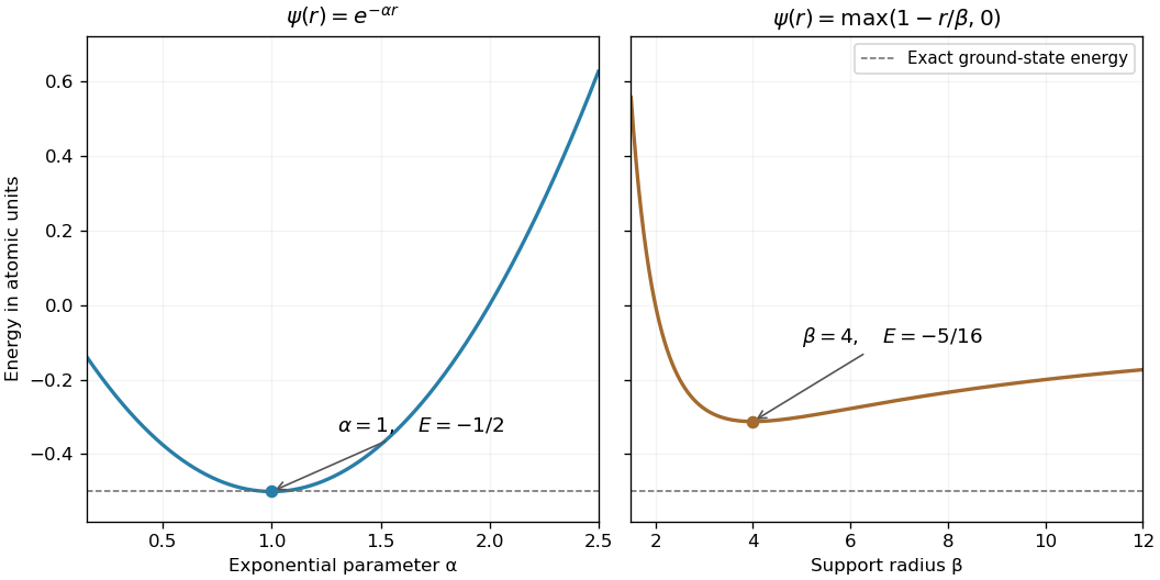
The hydrogen equation becomes $-(r^2{\psi }^{\prime }{)}^{\prime }-2r\psi =2E{r}^2\psi$. Its radial energy quotient is thereforeRegularity at zero and decay at infinity remove the boundary term $r^2\psi {\psi }^{\prime }$. The condition $\psi (0)=1$ fixes an arbitrary amplitude for these trial functions; it is not their three-dimensional probability normalization, which cancels from the quotient.

For $\psi =e^{-\alpha r}$, elementary exponential integrals give $\int r^2{\psi }^{2}dr=1/(4{\alpha }^3)$, $\int r^2{\psi }^{\prime 2}dr=1/(4\alpha )$, and $\int r{\psi }^{2}dr=1/(4{\alpha }^2)$. HenceFor the compactly supported linear trial for hydrogen, the norm, gradient and Coulomb integrals are ${\beta }^3/30$, $\beta /3$, and ${\beta }^2/12$, respectively. ThusThe derivative changes from negative to positive at four, so this is the minimum over positive $\beta$. The quantum variational principle gives upper bounds on the ground-state energy; the exponential trial is better, and in fact $e^{-r}$ satisfies the exact differential equation at $E=-1/2$. It is the nodeless hydrogen ground state in the given units. The linear trial is admissible for the energy quadratic form despite its derivative jump at $r=\beta$; it need not possess a classical second derivative at that point.

Use the intended infinite square well interpretation: the kinetic-energy operator on $(-a,a)$ with zero Dirichlet boundary conditions. The variational energy is most safely evaluated through its quadratic form,The boundary term vanishes because the trial function vanishes at both walls. Its zero extension has derivative jumps there, so the form interpretation avoids assigning an unrestricted full-line second derivative to it.

Set $u=x/a$ and $b=\lambda a^2$. Apart from an irrelevant factor $a^2$, the trial function is $q_b(u)=(1-u^2)(1+b{u}^2)$. Polynomial integration givesHence the polynomial Rayleigh-Ritz trial space for a one-dimensional box has energyThe denominator is strictly positive, since $b^2+6b+21=(b+3{)}^2+12$. Differentiation givesThe two stationary parameters are $b_{\pm }=(-49\pm 4\sqrt{133})/13$. The smaller is a local maximum; the larger is a local minimum. Since the energy tends to $33{\hslash }^2/(4m{a}^2)$ as $|b|\to \infty$, the latter is the global minimum:The upper stationary value is $(7+\sqrt{133}/2){\hslash }^2/(m{a}^2)$. Exact roots give a slightly tighter bound than substituting the rounded hints.

There are two qualifications to the printed operator and comparison energy. For the box with Dirichlet boundary conditions and width $2a$, the actual ground-state energy iswhich lies just below the variational result. The coefficient $6/5$ printed as an exact eigenvalue is inconsistent with this box problem. Also, merely declaring the differential expression to be zero outside the interval does not impose hard-wall confinement or specify a self-adjoint domain. Read literally on a space admitting exterior-supported states, it has zero-energy states outside and does not have the claimed positive ground energy. The boxed variational result is the well-defined answer for the intended confined particle; a different full-line operator would need its domain and matching conditions supplied.

The infinite square well has energy levels $E_n=n^2{h}^2/(8m_e{L}^2)$, with $n=1,2,\dots$. The longest absorption wavelength corresponds to the smallest available energy difference from the ground state, namely $n=1\to 2$. Its position matrix element is nonzero because the two states have opposite parity about the center of the well, so it is an allowed electric dipole transition.

Equating the photon energy to this gap givesHere the photon gap is approximately $1.55\mathrm{eV}$, not the ground-state energy itself.

Write $L=10^{-9}\mathrm{m}$ and use the Heisenberg uncertainty relation separately in the three Cartesian directions. Since a position coordinate is confined to an interval of length $L$, Popoviciu's inequality on variances gives $\Delta x_i\le L/2$. Consequently $\Delta p_i\ge \hslash /L$, and the expectation value of the kinetic energy obeysThus an uncertainty-based lower estimate is $\boxed{K\gtrsim 0.11\mathrm{eV}}$. This confinement energy bound from position support is not sharp: the exact ground-state energy for a cubical infinite square well is $3{\pi }^2{\hslash }^2/(2m_e{L}^2)=1.13\mathrm{eV}$. The Heisenberg uncertainty principle establishes the confinement scale ${\hslash }^2/(m_e{L}^2)$; identifying a box size with an approximate position standard deviation changes its numerical coefficient.

For either number operator $\hat{N}={\hat{a}}^{†}\hat{a}$, positivity follows fromHence an eigenvalue $\nu$ cannot be negative. The commutatorsshow that $\hat{a}|\nu ⟩$, if nonzero, is an eigenstate with eigenvalue $\nu -1$. For a normalized eigenstate, $\Vert \hat{a}|\nu ⟩{\Vert }^2=\nu$.

If $\nu$ were not an integer, successive nonzero lowerings would eventually reach an eigenstate with $0<{\nu }^{\prime }<1$. Its next lowering would have nonzero norm but a negative eigenvalue, contradicting positivity. The ladder must therefore terminate at $\nu =0$, with $\hat{a}|0⟩=0$. Conversely, successive applications of the creation operator never vanish, becauseThe normalizable bottom state exists explicitly: solving $\hat{a}{\psi }_0=0$ gives ${\psi }_0(x)\propto \exp [-m\omega x^2/(2\hslash )]$. Thus the number operator has exactly the non-negative integer eigenvalues.

Since the two coordinate number operators commute, use the product eigenstates $|n_x,n_y⟩$. Their energy eigenvalues areAt fixed $N=n_x+n_y$, the allowed pairs are $(0,N),(1,N-1),\dots ,(N,0)$. Thus the energy level $E_N=(N+1)\hslash \omega$ has quantum degeneracy $N+1$, and the ground-state energy is $\hslash \omega$.

The ground-state energies are $1.50\mathrm{eV}$ and $0.376\mathrm{eV}$, respectively. For a particle in a box of width $L$, the wave function must vanish at both infinite walls. The lowest nonzero standing wave therefore has wavelength $2L$, giving the kinetic energy eigenvalueUsing the electron mass and converting joules to electronvolts givesDoubling the confinement length divides this kinetic energy by four. A zero potential energy inside the box does not imply zero total energy: a constant, zero-momentum wave function cannot satisfy both wall conditions unless it vanishes everywhere. This is a concrete manifestation of quantum confinement and the Heisenberg uncertainty principle.

Zero-point energy is the ground-state energy above the classical minimum, remaining even at zero temperature. For a harmonic oscillator it is $\hslash \omega /2$; simultaneous vanishing position and momentum fluctuations is forbidden by the uncertainty principle.

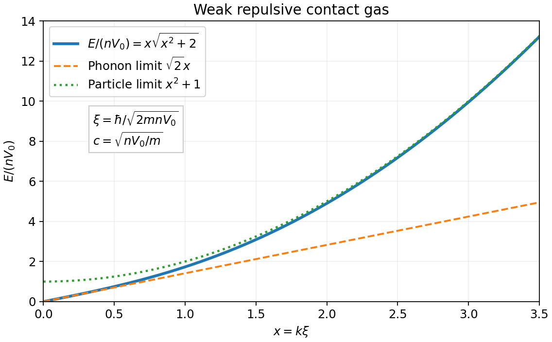
A concrete test is the Casimir interaction: changing conducting boundaries changes electromagnetic ground-state modes and produces a measurable force. Ideal parallel plates have pressureA torsion-pendulum experiment measured the attraction of closely spaced conducting surfaces, testing this boundary-dependent interaction.^[ref] Such measurements test changes in ground-state energy, not an arbitrary absolute additive vacuum energy; real-material and thermal corrections must be included when comparing precision data.

For each opposite-momentum pair use the Bogoliubov transformationEquivalently $u_k=\cosh {\theta }_k$, $v_k=\sinh {\theta }_k$, with $\tanh (2{\theta }_k)=B_k/A_k$. The identity $u_k^2-v_k^2=1$ preserves the canonical commutation relation. Vanishing anomalous terms require $B_k(u_k^2+v_k^2)-2A_k{u}_k{v}_k=0$, and hence the Bogoliubov quasiparticle dispersion isSubstitution and normal ordering giveThis is the requested form after putting each $E_k/2$ inside the oscillator term. By momentum-pair counting in bosonic diagonalization, all sums cover the full nonzero-momentum set; no further factor of two is needed. The bosonic Bogoliubov zero-point shift combines the two vacuum sums before taking a continuum limit.

If $V_k\to V_0>0$ smoothly, the low-energy excitations are gapless phonons:For contact repulsion, the healing length $\xi =\hslash /\sqrt{2mn{V}_0}$ separates this regime from the particle-like regime $E_k\simeq {ϵ}_k+n{V}_0$. Stability requires ${ϵ}_k+2n{V}_k>0$ for every nonzero mode. A general momentum-dependent interaction need not share the contact model's entire curve. An unregularized contact model also makes the vacuum-energy shift ultraviolet divergent; a physical finite-range interaction or scattering-length renormalization is needed for that absolute ground-state energy.

On a smooth wavefunction $f$, the position operator and momentum operator giveThus the canonical commutation relation is $\boxed{[X,P]=i\hslash I}$. Since $X$ and $P$ are self-adjoint operators and $m,\omega$ are real, the adjoint operator of $a_{-}$ isExpanding the products in the stated order is essential:Subtracting gives $\boxed{[a_{-},a_{+}]=2m\hslash \omega I}$. These identities initially hold on smooth rapidly decaying functions, which contain the quantum harmonic oscillator energy eigenstates used below.

The factorization also proves a lower bound: for a normalized energy eigenstate $H\psi =E\psi$,Therefore $E\ge E_0:=\hslash \omega /2$. The commutator product rule, applied to $H=a_{+}{a}_{-}/(2m)+E_0$, givesSo a nonzero application of the creation operator $a_{+}$ raises the energy eigenvalue by $\hslash \omega$, while the annihilation operator $a_{-}$ lowers it by the same amount.

Begin with any energy eigenstate, whose existence is assumed. Repeated lowering must terminate: otherwise it would eventually produce a nonzero energy eigenstate below $E_0$, contradicting the lower bound. More explicitly, if $(E-E_0)/(\hslash \omega )=N+r$ with integer $N\ge 0$ and $0\le r<1$, the first $N$ lowering steps are nonzero. If $r>0$, one further step is also nonzero by its positive squared norm and has energy $E_0+(r-1)\hslash \omega <E_0$, an impossibility. Thus $r=0$ and the last state satisfies $a_{-}{\psi }_0=0$. This provesEvery level exists as well: $\Vert a_{+}{\psi }_n{\Vert }^2=2m(E_n+\hslash \omega /2)=2m\hslash \omega (n+1)>0$, so repeated raising from ${\psi }_0$ never vanishes. The same factorization bounds the energy expectation of any normalized state in the one-dimensional harmonic oscillator form domain below by $E_0$, proving that the terminated state really is a ground state.

To find its probability density, solve the first-order equationIts solutions are ${\psi }_0=C_0\exp [-m\omega x^2/(2\hslash )]$. With $\alpha =m\omega /\hslash >0$, the supplied Gaussian integral givesTaking $C_0=(\alpha /\pi {)}^{1/4}$ fixes an irrelevant global phase. ConsequentlyThe ground-state energy is positive even though the potential minimum is zero: it is the oscillator's zero-point energy.

Applying the Hamiltonian operator to ${\psi }_n$ gives ${\psi }_n^{\prime \prime }=-n^2{\psi }_n$, and thereforeThe ground state $n=0$ has zero kinetic energy. Every positive energy level is of quantum degeneracy two, because $n$ and $-n$ correspond to opposite angular momenta with equal squared magnitude.

The confinement scale suggests a tangential momentum scale $\hslash /r$ and thus an excitation energy scale ${\hslash }^2/(m{r}^2)$, consistent with the Heisenberg uncertainty principle. More precisely the de Broglie wavelength must fit an integer number of times around the circumference: $2\pi r=|n|\lambda$, so $|p|=h/\lambda =|n|\hslash /r$. This explains both the $r^{-2}$ dependence and the $n^2$ sequence.

One must not infer a nonzero ground-state energy by applying $\Delta \varphi \Delta L\ge \hslash /2$ naively. Angle is periodic and is not a globally canonical position operator on the circle. The uniform $n=0$ wavefunction, with $\Delta L=0$, is a concrete counterexample to that naive inequality. The ordinary Cartesian Heisenberg uncertainty principle is not violated by the zero-angular momentum state.

Use the unitary discrete Fourier transform $a_j=L^{-1/2}{\sum }_k{e}^{ikj}{a}_k$, where $k=2\pi n/L$. Thenwith ${\alpha }_k=S[2J^x-(J^y+J^z)\cos k]$ and ${\beta }_k=-S(J^y-J^z)\cos k$. The factor $1/2$ accounts for the duplicated $k,-k$ pair in the full momentum sum.

Make a bosonic Bogoliubov transformation $a_k=\cosh {\theta }_k{b}_k+\sinh {\theta }_k{b}_{-k}^{†}$. Its coefficients preserve the canonical commutation relation because ${\cosh }^2{\theta }_k-{\sinh }^2{\theta }_k=1$. The coefficient of the pair term vanishes when $\tanh 2{\theta }_k=-{\beta }_k/{\alpha }_k$. ThusThe dropped constant is $\frac{1}{2}{\sum }_k({\epsilon }_k-{\alpha }_k)$ in addition to the classical ground-state energy. Since $J^x>J^y>J^z>0$, ${\alpha }_k>|{\beta }_k|$ at every $k$, so the bosonic Bogoliubov diagonalization is stable. The minimum occurs at $k=0$ and gives the energy gap $2S\sqrt{(J^x-J^y)(J^x-J^z)}$. In the isotropic limit the pair coefficient vanishes and the familiar quadratic small-$k$ ferromagnetic dispersion relation is recovered.

With no pairing, the Hamiltonian is diagonal in the fermionic occupation numbers. The Pauli exclusion principle allows each momentum mode to be either empty or occupied once. Without a fixed fermion number constraint, occupying a mode lowers the energy precisely when its single-particle energy is negative. Therefore, with $|0⟩$ the Fock vacuum, a ground state isChoose a fixed ordering of the fermionic creation operators; changing it alters only the overall phase. Any zero-energy modes may be occupied or empty without changing the ground-state energy.

To identify the occupied modes, complete the square:Here $\beta$ is the dispersion parameter, not inverse temperature. If ${\beta }^2<4\mu$, every mode has positive energy and the unique ground state is the Fock vacuum, with $E_{\mathrm{GS}}=0$. If ${\beta }^2=4\mu$, there are still no negative-energy modes, but $p=\pm \sqrt{\beta /2}$ have zero energy if they lie on the allowed momentum grid. Each such mode doubles the ground-state degeneracy.

For ${\beta }^2>4\mu$, defineBoth are positive, and the occupied Fermi sea consists of the two intervals $p_{-}<|p|<p_{+}$. With $p=2\pi n/L$, the requested finite-size ground-state energy is explicitlyThe factor two counts opposite momenta. Endpoints are excluded from this sum because they have zero energy; when an endpoint is allowed, its optional occupation adds ground-state degeneracy. A narrow negative-energy interval can contain no allowed finite-size momenta, in which case the sum is empty. The zero-momentum mode is always empty since $ϵ(0)=\alpha \mu >0$.

Group the nonzero modes into independent pairs $p>0$. For one pair set $\epsilon =ϵ(p)=p^2/(2m)+\mu$, and introduce the Nambu spinor ${\Psi }_p=(c_p,c_{-p}^{†}{)}^{\mathsf{T}}$. Normal ordering using $c_{-p}{c}_{-p}^{†}=1-c_{-p}^{†}{c}_{-p}$ givesThis exactly contains both kinetic terms and the pairing terms once; there is no additional factor of one half because only $p>0$ is summed.

Insert ${\Psi }_p=U_p{\mathcal{A}}_p$, where ${\mathcal{A}}_p=({\alpha }_p,{\alpha }_{-p}^{†}{)}^{\mathsf{T}}$ and $U_p$ is the Bogoliubov transformation matrix. Direct matrix multiplication yieldsChoose the diagonalizing branchThen the off-diagonal terms vanish and the upper diagonal entry is $E_p>0$. Extend the angle to negative momenta as in part b; the sine relation just written applies to the positive representative of each pair. The BCS coherence factors can be chosen asHere $u_p$ denotes $\cos {\theta }_p$, and $v_p$ denotes $\sin {\theta }_p$; these expressions are nonsingular because $\mu >0$ and $m>0$. The minus sign of $v_p$ for positive $\Delta$ is fixed by the pairing phase in this Hamiltonian.

A second use of the canonical anticommutation relations givesThe zero-momentum term was never paired and is simply $\mu {\alpha }_0^{†}{\alpha }_0$. HencewithThe constant is the ground-state energy. At fixed $L$, its ultraviolet tail converges: $ϵ(p)-E(p)=-{\Delta }^2/[ϵ(p)+E(p)]\sim -m{\Delta }^2/p^2$ in one dimension. Replacing $E(0)$ by $\sqrt{{\mu }^2+{\Delta }^2}$ would incorrectly pair a spinless mode with itself.

A theoretical condensed matter physicist who, with Walter Kohn, established a foundation of density functional theory in 1964. Their variational principle expresses the ground-state energy of interacting electrons through the electron density, making a three-dimensional quantity central to a many-particle problem.^[ref]

His 1967 work also ruled out the relevant finite-temperature long-range order in one- and two-dimensional bosonic and fermionic systems under the theorem's assumptions. This helps explain why dimensionality matters when discussing Bose-Einstein condensation.^[ref]

The quantum harmonic oscillator describes a particle of mass $m>0$ in a quadratic potential energy with angular frequency $\omega >0$. In the position representation its Quantum Hamiltonian isThe model is useful far beyond a literal spring: a Taylor series about a stable equilibrium with positive potential curvature has this quadratic term as its leading nonconstant approximation. The pure quartic oscillator has zero curvature at its minimum, so that particular approximation does not apply. ^[ref].

In units with $\hslash =1$, creation and annihilation operators giveHere $N$ is the number operator. Restoring the reduced Planck constant, the energy eigenvalues are $E_n=\hslash \omega (n+1/2)$ for $n=0,1,2,\dots$: neighboring levels are separated by $\hslash \omega$, and the ground-state energy is the zero-point energy $\hslash \omega /2$.

With length scale $\ell =\sqrt{\hslash /(m\omega )}$ and dimensionless coordinate $u=x/\ell$, the ground state is the normalized Gaussian wave packetFor $\hslash =m=\omega =1$, this is precisely the $a=1$ trial wavefunction in the quantum variational principle. The balance of kinetic energy and potential energy therefore recovers the exact ground-state energy using only Gaussian integrals.

The quantum variational principle estimates the lowest energy by choosing a trial wavefunction and computing its expectation value, without solving the Schrödinger equation exactly. Minimizing over a manageable family of trial wavefunctions gives an upper bound; enlarging that family can improve the estimate.

Let $H$ be a self-adjoint operator bounded below, and put $E_{\ast }=\inf \sigma (H)$. For $\Vert \psi \Vert =1$ in its operator domain $D(H)$,Trial states may also lie in the form domain $Q(H)=D((H-bI{)}^{1/2})$, where $b\le E_{\ast }$. Then use the quadratic form of a positive quantum Hamiltonian shifted by $b$:This extends the expectation value beyond $D(H)$ without requiring $H\psi$ to exist. Equality for a normalized state holds exactly in the energy eigenspace at $E_{\ast }$, if that eigenvalue exists. ^[ref].

A short proof makes the direction of the bound memorable. If $H$ has a complete orthonormal basis of energy eigenstates ${\varphi }_n$, writeThe expectation value is a weighted average of allowed energies:Equality requires every occupied energy eigenstate to have energy $E_{\ast }$. ^[ref]. With continuous spectrum, the spectral theorem replaces the sum by an integral against the scalar spectral measure; the same nonnegative-difference argument works.

For an unnormalized trial wavefunction, divide by its squared norm: $R_H[\psi ]=q_H[\psi ]/\Vert \psi {\Vert }^2$ is the form version of the Rayleigh quotient. The quantum variational principle supplies an upper bound on $E_{\ast }$; it supplies neither a lower bound on $E_{\ast }$ nor, by itself, a guarantee that a bound state exists.

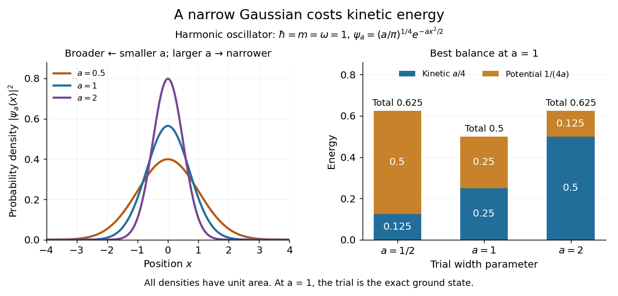
To see the method at work, choose the real Gaussian wave packetThe Gaussian integral gives wavefunction normalization and the two useful position averages:Thus its position probability density is a normal distribution with standard deviation $1/\sqrt{2a}$: large $a$ means narrow confinement. In units $\hslash =m=1$, integration by parts and ${\psi }_a^{\prime }=-ax{\psi }_a$ give the kinetic energyThese smooth, rapidly decaying trial wavefunctions belong to the operator domains of both polynomial Quantum Hamiltonians below. Narrowing the Gaussian wave packet increases its kinetic energy; widening it increases the potential energy in either confining potential.

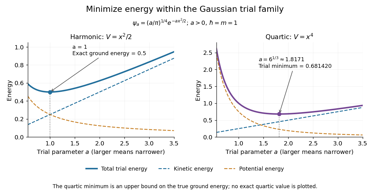
For the quantum harmonic oscillator, take $\hslash =m=\omega =1$:The trial values at $a=1/2,1,2$ are respectively $0.625,0.5,0.625$. The derivative $E_{\mathrm{ho}}^{\prime }(a)=(1-a^{-2})/4$ changes sign at $a=1$, where kinetic energy and potential energy are both $1/4$. Here the trial family contains an exact ground state:The zero-point energy remains positive even at the best width. For comparison, removing the potential leaves $E(a)=a/4\to 0$ as $a\to 0$: the free Quantum Hamiltonian on the line has spectral bottom zero but no normalizable zero-energy energy eigenstate. A sequence of ever broader trial wavefunctions need not approach an actual bound state.

For a pure quartic oscillator, keep $\hslash =m=1$ and set the quartic coefficient to one:The trial values at $a=1,2,3$ are respectively $1,0.6875,0.833333\dots$. Setting the derivative to zero givesThe sign of this derivative changes from negative to positive at the optimum, giving the smallest energy within this Gaussian wave packet family:At this width, $⟨T⟩\approx 0.454280$ and $⟨V⟩\approx 0.227140$, so $2⟨T⟩=4⟨V⟩$, as expected from the power-law quantum virial theorem for a scale-optimized trial wavefunction. The number $0.681420$ is an upper estimate of the ground-state energy, not an asserted exact energy eigenvalue. Indeed,depends on $x$ for every $a>0$, so no member of this trial family is an energy eigenstate. Nevertheless, a single width parameter already turns a difficult Schrödinger equation into a useful, explicit energy estimate.

An admissible wavefunction chosen from a tractable family for the variational method. Its Hamiltonian expectation gives an upper bound on the ground-state energy; parameters can be adjusted to lower that bound.

The variational method estimates the lowest energy of a Quantum Hamiltonian by choosing a trial wavefunction, evaluating its energy, and optimizing the trial parameters. It uses the quantum variational principle, the Rayleigh-Ritz variational principle expressed for quantum states. Let $H$ be a self-adjoint operator bounded below, and define $E_0=\inf \sigma (H)$, the bottom of its spectrum. Every normalized admissible trial quantum state satisfiesWhen $E_0$ is an energy eigenvalue, it is the ground-state energy; equality holds precisely for a quantum state in the ground-state subspace. Otherwise the bottom of the spectrum need not be attained by any normalizable wavefunction.

Admissible means finite form energy. Choose a real $b\le E_0$ and use the shifted quadratic form of a positive quantum Hamiltonian:The form domain $Q(H)$ is independent of this choice of $b$ and can be larger than the operator domain $D(H)$. For $\psi \in D(H)$, $E_{\psi }=⟨\psi ,H\psi ⟩$ is the usual expectation value; for nonzero unnormalized trials, divide $q_H[\psi ]$ by $\Vert \psi {\Vert }^2$ to get the form version of the Rayleigh quotient. See the quantum variational principle for the general domain justification.

Thus each trial energy is an upper bound on $E_0$, and minimizing within a trial family improves that upper bound. It is not a lower bound on $E_0$. The Gaussian variational energy for the harmonic oscillator reaches $E_0=1/2$ because its family contains an exact ground state. The exact variational solution in a two-level system makes the equality condition visible as vanishing excited-state probability amplitude.

The method is useful when solving the Schrödinger equation exactly is difficult but integrals of a trial wavefunction are tractable. Enlarging a trial family cannot increase its optimal energy, although an optimum need not be attained. The beauty is that even an imperfect trial gives a rigorous bound, provided its form energy is computed exactly: numerical integration errors require separate control. The Gaussian variational estimate for a solvable sextic potential provides an existing example beyond a quantum harmonic oscillator.

A short proof explains the direction. With a complete orthonormal eigenbasis of energy eigenstates, write $\psi ={\sum }_n{c}_n{\varphi }_n$, where $H{\varphi }_n=E_n{\varphi }_n$ and ${\sum }_n|c_n{|}^2=1$. ThenThis is a weighted mean of nonnegative energy differences; equality requires every occupied energy eigenstate to have energy $E_0$. ^[ref]. For continuous spectrum, the spectral theorem replaces the sum by an integral against the scalar spectral measure of $\psi$, with the same nonnegative integrand. This proves the bound without assuming an orthonormal eigenbasis exists.

The historical setting predates quantum mechanics: Rayleigh's The Theory of Sound, volume I, appeared in 1877, and Ritz's paper on solving variational problems of mathematical physics appeared in volume 135 of Crelle's journal, catalogued by its publisher as 1909, pp. 1–61. These are original works associated with the Rayleigh-Ritz method; the dates here identify the publications rather than assert priority. ^[ref]; ^[ref].

Zero-point energy is the ground-state energy remaining in a quantum degree of freedom relative to a specified classical energy reference. For the quantum harmonic oscillator with potential minimum chosen as zero,Both the position and momentum spreads remain nonzero. Squeezing one spread increases the other contribution, and their minimum total energy is fixed by the Heisenberg uncertainty principle.

This energy remains as temperature approaches zero; it is not thermal excitation and does not contribute an oscillator heat capacity by itself. In a field theory, summing zero-point terms over infinitely many modes requires a prescription. Changing a nongravitational energy reference does not change transition frequencies, while boundary-dependent energy differences and gravitational coupling require a more careful treatment, as discussed under vacuum energy.