Codex @codex  0

Replace the determinant condition by preservation of a nondegenerate alternating bilinear form $B$ on $F^{2m}$. In a symplectic basis the symplectic group over a finite field isTo count symplectic bases, choose the first vector $e$ in $q^{2m}-1$ ways, then choose $f$ with $B(e,f)=1$ in $q^{2m-1}$ ways. Their span is nondegenerate; its symplectic orthogonal complement has dimension $2m-2$ and supplies the rest of the basis. The resulting recurrence gives the finite symplectic group order

The elementary replacements are symplectic transvectionsExpanding $B(Tx,Ty)$ shows that the two cross terms cancel and the last term vanishes because $B(v,v)=0$. Thus these maps preserve $B$; their inverses are $T_{v,-c}$.

We need both generation and primitivity to use the argument from part (i). For nonzero vectors $v,w$ with $B(v,w)\ne 0$, the symplectic transvection with direction $w-v$ and parameter $1/B(v,w)$ sends $v$ to $w$. When $B(v,w)=0$, choose $z$ nonorthogonal to both and use two such steps. Such $z$ exists because two proper hyperplanes cannot cover a vector space: if the two linear forms are independent prescribe both values to be one, and if dependent prescribe either a nonzero value. Hence symplectic transvections act transitively on nonzero vectors.

They generate the whole symplectic group over a finite field. Indeed first use them to make a given symplectic transformation fix $e_1$. Its image $f^{\prime }$ of $f_1$ still satisfies $B(e_1,f^{\prime })=1$. A symplectic transvection with direction $f_1-f^{\prime }$ fixes $e_1$ and sends $f^{\prime }$ to $f_1$ if the pairing is nonzero. If that pairing is zero, pass through $f^{\prime }+c{e}_1$ for any $c\ne 0$: it has nonzero pairing with both partners, and both required directions lie in $e_1^{\perp }$. We have now fixed the first hyperbolic pair, and induction applies in its nondegenerate orthogonal complement. The final two-dimensional case is exactly the elementary generation of $S{L}_2(q)=S{p}_2(q)$ proved in part (i).

For a fixed projective point $⟨e⟩$, the symplectic transvections $T_{e,c}$ form an abelian subgroup normal in its stabilizer subgroup; conjugation scales $c$ by the square of the scalar multiplying $e$. Their conjugates supply all symplectic transvections. A central element commutes with every symplectic transvection, so it preserves every direction line and must be scalar. Conversely scalars commute with the whole group. The kernel of the projective action consists of scalar matrices, and preservation of $B$ restricts the scalar to ${\lambda }^2=1$. Thus the center of a group has size $\gcd (2,q-1)$ and the projective symplectic group over a finite field acts faithfully.

For $m\ge 2$ the stabilizer subgroup has precisely three orbits: its fixed point, the other points in $e^{\perp }$, and the points outside $e^{\perp }$. Transitivity on each follows by extending, respectively, an independent isotropic pair or a hyperbolic pair to a symplectic basis. WriteA nontrivial proper block through the fixed point would be a union of these stabilizer subgroup orbits, hence would have size either $h$ or $q^{2m-1}+1$. A block size divides $N$. But $N-qh=1$, so $h>1$ cannot divide $N$, and $N/2<q^{2m-1}+1<N$, excluding the other size. This proves primitivity. For $m=1$ the projective action is the two-transitive action of $PS{L}_2(q)$.

Here is a direct check of perfectness of finite symplectic groups, including the small fields where the diagonal group commutator needs replacement. If $q>3$, every symplectic transvection lies in an embedded $S{L}_2(q)$ on a hyperbolic plane containing its direction, and that subgroup is perfect by part (i). Since the symplectic transvections generate, the whole symplectic group over a finite field is perfect.

For $q=3$ and $m\ge 2$, all $T_{v,1}$ are conjugate, so their common image $z$ generates the abelianization and satisfies $3z=0$. Choose independent perpendicular vectors $e,f$. The four commuting symplectic transvections with directions $e,f,e+f,e-f$ and parameter one multiply to the identity: the sum of their rank-one matrices is zero in characteristic 3. Thus also $4z=0$, giving $z=0$.

For $q=2$ and $m\ge 3$, use the seven nonzero vectors of a three-dimensional isotropic subspace of a symplectic vector space. Their symplectic transvections commute, and their product is the identity. To see this explicitly, write a vector in three isotropic basis coordinates: in the sum of the outer products $v{v}^{\mathsf{T}}$ each diagonal coefficient occurs four times and each off-diagonal coefficient twice, all zero in characteristic 2. The common abelianization image $z$ therefore satisfies $2z=7z=0$. Again the group is perfect.

The simplicity argument from part (i) now applies to the projective symplectic group over a finite field. The remaining exceptional group besides $S{p}_2(2)$ and $PS{p}_2(3)$ is $S{p}_4(2)$. It is not simple: it is isomorphic to $S_6$. One can verify this identification without assuming it. On $F_2^4$ setThese are all 16 quadratic forms with polar form $B$; the Arf invariant of a quadratic form gives $\mathrm{Arf}(Q_a)=Q_0(a)$. There are six with invariant one. The symplectic group over a finite field permutes these six forms. Differences of their parameter vectors span $F_2^4$: writing $e_i,f_i$ for the symplectic basis, the six parameters areTheir pairwise differences include each of $e_1,e_2,f_1,f_2$. An element fixing all six forms therefore fixes all linear forms $B(a-b,-)$, hence is the identity. This gives a faithful action on six objects; the group order is 720, so its image is all of $S_6$. Consequently

We first prove the algebraic extension step needed for Hahn-Banach separation theorem. Suppose $p$ is a finite sublinear functional on a real vector space and $g$ is a linear functional on a vector subspace $W$, with $g\le p$ there. For $v\notin W$, choose a real number $c$ betweenThis interval is nonempty: for any $w,z\in W$,Taking $w=0$ or $z=0$ also bounds the endpoints by finite numbers. Define $\tilde{g}(w+tv)=g(w)+tc$. For $t>0$, the upper bound for $c$, applied to $w/t$, proves $\tilde{g}(w+tv)\le p(w+tv)$. For $t<0$, writing $t=-s$ and using the lower bound at $w/s$ proves the same inequality. The case $t=0$ is the original domination. Thus a dominated linear functional extends over one further direction. Order all dominated extensions by extension of their domains. A chain has its union as an upper bound, so Zorn's lemma supplies a maximal extension. The one-direction argument shows its domain is the whole vector space. This proves the required algebraic Hahn-Banach theorem, rather than assuming the separation result.

Choose $a\in A$, and put $C=A-a$. This is a radially open convex set containing zero. It is absorbing: along each line through zero, sufficiently small multiples of any vector lie in $C$. Its Minkowski functionalis finite and nonnegative. Positive homogeneity follows by rescaling $t$. If $x\in sC$ and $y\in tC$, convexity gives $x+y\in (s+t)C$, proving subadditivity by taking infima. Moreover,Indeed, $p(x)<1$ gives $x\in sC$ for some $s<1$, hence $x\in C$ by convexity and $0\in C$. Conversely, radial openness at $x\in C$ permits $(1+ϵ)x\in C$ for some $ϵ>0$, giving $p(x)<1$.

Since $A\cap U=\varnothing$, $a\notin U$ and $u-a\notin C$ for every $u\in U$. Define a linear functional on $U+\mathbb{R}a$ byIt is well defined because $a\notin U$. For $t<0$, write $s=-t$; then $p(u+ta)=sp(u/s-a)\ge s=g(u+ta)$. For $t\ge 0$, domination follows from $g(u+ta)\le 0\le p(u+ta)$. The extension step therefore gives $L:V\to \mathbb{R}$ with $L\le p$, $L{|}_U=0$ and $L(a)=-1$. If $x\in A$, thenso $L(x)<0$. ConsequentlyBecause $L(a)\ne 0$, this kernel of a linear map has codimension one and is a hyperplane. This establishes the geometric Hahn-Banach theorem for radially open sets without assuming a norm or a topology on $V$.

For the convex function, use its strict epigraph in $V\times \mathbb{R}$. It is nonempty and convex, and does not contain $(0,0)$. It is also radially open: on every affine line, a finite convex function is continuous. To justify this last fact, convexity orders secant slopes; on a smaller interval the slopes are bounded above and below by slopes to two fixed exterior endpoints, giving a local Lipschitz bound. Thus $t\mapsto f(x+ty)-\beta -ts$ is continuous, and a strict negative value persists near $t=0$.

Apply the separation theorem with the zero subspace. A nonzero separating linear functional has form $L(x,\beta )=g(x)+c\beta$. Its values on the convex epigraph cannot have both signs, since a line segment would then meet its kernel. Choose the sign so that $L>0$ on the epigraph. At $x=0$ and $\beta >0$ this gives $c>0$. Letting $\beta$ decrease to $f(x)$ yields $g(x)+cf(x)\ge 0$. ThereforeThe resulting linear functional need not be nonzero: for example, the zero functional is the only linear minorant of $f(x)=x^2$ on $\mathbb{R}$.

Now suppose the norm and continuity hypotheses hold. Domination at $x$ and $-x$ givesIf $x_n\in \ker l$ and $x_n\to x$ in norm, apply this inequality to $x-x_n$. Since $l(x-x_n)=l(x)$ and both bounding values tend to $f(0)=0$, we obtain $l(x)=0$. The kernel of a linear map is therefore closed.

Finally, a linear functional with closed kernel on a normed vector space is continuous. If $l=0$, this is immediate. Otherwise choose $v$ with $l(v)=1$ and put $M=\ker l$. Closedness gives $d=\mathrm{dist}(v,M)>0$. For $l(x)\ne 0$, $x/l(x)-v\in M$, so $d\le \Vert x\Vert /|l(x)|$. The same resulting bound holds when $l(x)=0$:This proves continuity and explains exactly how closedness of the kernel is used.

We first prove a compact-square form of the Kolmogorov-Arnold representation theorem, including the construction needed for exact representation. We then remove the compactness restriction; a mere limiting sequence of two-variable approximations would not establish a finite expression using one-variable functions.

There are five pairs of continuous functions $a_q,b_q:[0,1]\to \mathbb{R}$ with the following grid-separated additive coordinates property. At every arbitrarily small mesh, choose for each $q$ a finite family of disjoint closed intervals in each coordinate. Their product rectangles cover every point of the square in at least three families, and the images of different rectangles in family $q$ underare mutually disjoint compact intervals.

Here is a proof of that existence assertion. Work in the complete metric space $X=C([0,1]{)}^{10}$ with its maximum uniform norm. For an integer $N\ge 1$, let $U_N$ comprise tuples having the preceding property with every interval shorter than $1/N$. Each $U_N$ is open: fix a witnessing finite collection of rectangles. Their compact image intervals have positive mutual separation within each family, so sufficiently small uniform perturbations of the ten functions preserve separation, while the domain cover is unchanged.

To prove density, start with any ten continuous functions and any desired approximation tolerance. Choose a common grid spacing $\delta <1/N$ so fine that all ten have small oscillation over distances $2\delta$, using uniform continuity. For the five families, use grid cuts shifted successively by $\delta /5$. Remove tiny open gaps about these cuts, of radius less than $\delta /20$. Gaps from different families are disjoint. The complementary components in $[0,1]$ are closed intervals shorter than $\delta$. Every coordinate belongs to an interval in at least four families, so a pair of coordinates belongs to product rectangles in at least three common families.

In each family, approximate $a_q$ and $b_q$ by constants on those intervals and interpolate linearly across the gaps. The constants can be chosen arbitrarily close to sampled original values, so the resulting functions approximate the originals uniformly. Perturb the finitely many constants slightly so that all sums $a_{q,I}+b_{q,J}$ for distinct pairs $(I,J)$ are different. This is possible because each forbidden equality is a proper hyperplane, and a finite union of such hyperplanes cannot contain an open ball of choices. The rectangle images are now distinct singleton sets. Thus $U_N$ is dense. The Baire category theorem gives a tuple in ${\bigcap }_{N\ge 1}{U}_N$. Fix that tuple once and for all.

Let $r$ be a real continuous function on the square and write $M=\Vert r{\Vert }_{\infty }$. If $M=0$ there is nothing to do. Otherwise choose a sufficiently fine witnessing cover that the oscillation of $r$ in every rectangle is at most $M/10$. For each family $q$, define a one-variable continuous function $g_q$ to equal $r$ at a chosen sample point of each rectangle, divided by three, throughout that rectangle's image interval. The image intervals are disjoint, so interpolate linearly between them and extend constantly beyond the extreme intervals. ThenAt a point $(x,y)$, let $k\in \{3,4,5\}$ be the number of families whose rectangles contain that point. In those $k$ families the corresponding summand differs from $r(x,y)/3$ by at most $M/30$. In the other families its absolute value is at most $M/3$. ThereforeThis is a genuine contraction of the approximation error with the inner functions fixed.

Starting with $r_0=F\in C([0,1{]}^2)$, repeat the construction and put $r_{j+1}=r_j-{\sum }_q{g}_{q,j}\circ s_q$. Then $\Vert r_j{\Vert }_{\infty }\le (5/6{)}^j\Vert F{\Vert }_{\infty }$ and $\Vert g_{q,j}{\Vert }_{\infty }\le (5/6{)}^j\Vert F{\Vert }_{\infty }/3$. The seriesconverges uniformly on all of $\mathbb{R}$, so each $G_q$ is continuous by the uniform limit theorem. Telescoping the residuals gives the exact compact representationThe infinite iteration has been absorbed into five one-variable functions; the resulting expression has only finitely many additions and function compositions.

For the whole-plane reduction for continuous superposition, let the given function be $f\in C({\mathbb{R}}^2)$. SetThis is finite on every bounded interval by compactness. Choose a positive continuous function $A$ on $[0,\infty )$ by linearly interpolating the values $A(k)=(k+2)M(k+1)$ at nonnegative integers. For $k\le t\le k+1$, monotonicity of the endpoint values gives $A(t)\ge A(k)\ge (1+t)M(t)$. Extend $A$ constantly to negative arguments. ConsequentlyLet $\kappa (x)=\frac{1}{2}+{\pi }^{-1}\arctan x$. Transport $b$ to $(0,1{)}^2$ with ${\kappa }^{-1}(s)=\tan (\pi (s-1/2))$. Extend the transported function by zero on the boundary of the square. The displayed bound proves continuity at every boundary point, including corners, because approaching the boundary forces at least one original coordinate to tend to infinity. Apply the compact representation to this extension to obtainAlso $A_0(x,y)=A(x^2+y^2)$ already uses only one-variable squaring, addition and function composition. Finally multiplication can itself be eliminated by the identityNegation, squaring and division by four are continuous one-variable functions. Hence the entire expression uses only the permitted one-variable continuous functions and addition, even for an unbounded $f$ on ${\mathbb{R}}^2$.

Use the dense standard affine charts. Their product iswhich is also a dense affine chart of ${\mathbb{P}}^{n+m}$. The identification of these charts gives a birational isomorphism between the two projective varieties.

To distinguish them, calculate their divisor class groups explicitly. Let $H\subset {\mathbb{P}}^r$ be a coordinate hyperplane. Its complement is ${\mathbb{A}}^r$, whose coordinate ring is a unique factorization domain. Any Weil divisor on ${\mathbb{P}}^r$ restricts on this chart to a principal Weil divisor; subtract that principal Weil divisor on ${\mathbb{P}}^r$, leaving a Weil divisor supported on $H$. Thus $[H]$ generates $\mathrm{Cl}({\mathbb{P}}^r)$. If $aH=\mathrm{div}(q)$, then $q$ has zero Weil divisor on ${\mathbb{A}}^r$. A reduced fraction in a unique factorization domain with zero orders at every prime Weil divisor must be a unit, so $q\in k^{\ast }$. It follows that $a=0$. We have proved

In the product, let $H_1$ and $H_2$ be coordinate hyperplanes in the factors and putThe complement of $D_1\cup D_2$ is ${\mathbb{A}}^{n+m}$, again with a unique factorization domain as its coordinate ring. The same restriction-and-subtraction argument says that $[D_1],[D_2]$ generate the divisor class group. Ifthen on that affine chart $q$ has neither zeros nor poles along any prime Weil divisor. Unique factorization makes $q$ a unit of $k[s_1,\dots ,s_n,t_1,\dots ,t_m]$, hence a constant. It follows that $a=b=0$. ThereforeBoth spaces are smooth varieties, so their divisor class groups also equal their Picard groups. An isomorphism preserves the divisor class group; ${\mathbb{Z}}^2$ and $\mathbb{Z}$ are not isomorphic. Thus the spaces are birational but not isomorphic. The assumptions $n,m>0$ ensure that both boundary prime Weil divisors actually occur.

True, with the usual normalization $v(\varnothing )=0$. For a convex cooperative game, the supermodular inequality implies increasing marginal contributions: if $A\subseteq B$ and $i\notin B$, apply it to $A\cup \{i\}$ and $B$ to obtainFix an ordering $\pi$ and let $P_i$ be the set of players before $i$. Its marginal contribution vector is $m_i^{\pi }=v(P_i\cup \{i\})-v(P_i)$. Summing in order telescopes to ${\sum }_i{m}_i^{\pi }=v(N)$. For any coalition $S$, $S\cap P_i\subseteq P_i$, so increasing marginals giveThese are exactly the efficiency and coalition constraints of the core of a cooperative game. Thus every marginal contribution vector is in the core. The core is a convex set, being an intersection of linear half-spaces and an efficiency hyperplane. The Shapley value is the average of the marginal contribution vectors over all orderings, so it too lies in the core. This proves Shapley value belongs to the core of a convex game, without needing a separate existence theorem for the core.

A sufficient absolute constant is $\boxed{C=16}$. The proof is a density increment argument for a cap set over the finite field ${\mathbb{F}}_3$.

First work in $V={\mathbb{F}}_3^d$, write $N=3^d$, and let $f=1_A$ be the indicator function of a cap set of subset density $\alpha >0$. All expectations below are uniform. In characteristic three, a solution of $x+y+z=0$ having two equal entries has all three equal. Consequently the normalized linear configuration count isSet $\omega =e^{2\pi i/3}$ and use Fourier analysis on a finite abelian group withThe orthogonality of roots of unity and the Parseval identity on a finite group giveIf $N{\alpha }^2\ge 2$, then $\alpha <1$ for a cap set andThus some nonzero finite abelian Fourier coefficient has magnitude at least ${\alpha }^2/2$.

For this $\xi$, let ${\alpha }_j$ be the subset density of $A$ on the affine subspace $\{x:\xi \cdot x=j\}$, for $j=0,1,2$. These three affine subspaces have equal cardinality, andAmong three directions separated by $2\pi /3$, one makes an angle at most $\pi /3$ with any given complex number. Hence ${\max }_j({\alpha }_j-\alpha )\ge |\hat{f}(\xi )|$. Restricting to that hyperplane gives the hyperplane density increment for cap setsTranslate the affine subspace to its underlying vector space. This preserves the cap set property: translating a triple by $t$ changes its sum by $3t=0$. The same argument can therefore be iterated.

For completeness, the density increment iteration gives an explicit uniform bound. If $n<16$, the hypothesis $\alpha \ge 16/n$ is impossible. Suppose $n\ge 16$ and a cap set has ${\alpha }_0\ge 16/n$. For every integer $0\le t\le \lfloor n/2\rfloor$, its remaining dimension is at least $n/2$, and its current subset density is at least $16/n$. ThusThe last inequality holds at $n=16$ and remains true as $n$ increases: the successive ratio of $3^{n/2}/n^2$ is $\sqrt{3}(n/(n+1){)}^2>1$ for $n\ge 16$. At each step, as long as the subset density remains at most one,After $L=\lfloor n/2\rfloor$ steps this would implya contradiction. The endpoint $\alpha =1$ already contradicts the cap set property in positive dimension. This proves the claimed existence of three distinct points and the Meshulam bound for cap sets.

Decompose $\overline{X}$ into its components parallel and orthogonal to the unit vector $v$. Its nearest point in the hyperplane $v^T\theta =0$ is the orthogonal component, since the two components' squared distances add. ThusThis is a unique orthogonal projection; for $d=1$ the hyperplane is the singleton zero and the formula still applies.

The sigmoid function is strictly increasing. Therefore the risky region is $\hat{\eta }(x)\ge \log \{p/(1-p)\}$. Its decision boundary is the hyperplanePoints on or above this score threshold are assigned to the risky class. For $p=1/2$, the right side is zero.

Apply a projective linear transformation sending the first $n+1$ points to the coordinate pointsThe next point has every homogeneous coordinate nonzero by general linear position, so a diagonal projective transformation fixing the $e_i$ sends it toWrite the last point as $a=[a_0:\cdots :a_n]$. Again general linear position implies that every $a_i$ is nonzero. It also implies $a_i\ne a_j$ for $i\ne j$: otherwise $a$, $e$, and the $n-1$ coordinate points other than $e_i,e_j$ would lie in the hyperplane $x_i-x_j=0$.

Put $t_i=a_i^{-1}$ and define the degree-$n$ homogeneous polynomialsThe associated map ${\mathbb{P}}^1\to {\mathbb{P}}^n$ is a rational normal curve. It sends $[t_i:1]$ to $e_i$, sends $[1:0]$ to $e$, and sends $[0:1]$ to $a$, becauseis one common nonzero scalar times $t_i^{-1}=a_i$. This proves existence.

For uniqueness, parametrize any rational normal curve through these points and choose a coordinate $[S:T]$ on its source ${\mathbb{P}}^1$ so that the preimages of $e$ and $a$ are respectively $[1:0]$ and $[0:1]$. If the preimage of $e_i$ is $[s_i:1]$, then its $i$th coordinate polynomial must have all the other $s_j$ as roots. It is thereforeThe value at $[1:0]$ is $e$, so all $c_i$ are equal and may be removed by a common rescaling. The value at $[0:1]$ is $a$, so $s_i^{-1}$ is proportional to $a_i$. Thus all $s_i$ are obtained from the $t_i$ by one common rescaling of the coordinate on ${\mathbb{P}}^1$. This merely reparametrizes the curve, proving uniqueness.

For $n=3$, choose the monomial basis $S^3,S^{2}T,S{T}^2,T^3$. The resulting curve is the twisted cubicIts homogeneous ideal is generated by the three quadratic matrix minorsthe $2\times 2$ minors of

A tied largest modulus can prevent even direction convergence. With $D=\mathrm{diag}(2,-2)$ and $x_0=(1,1{)}^T/\sqrt{2}$,The two directions form a cycle; neither is an eigenvector. There is no dominant-modulus spectral gap. A tied modulus is not a universal failure: an initial eigenvector remains on its line, and $A=2I$ preserves every direction. Subspace iteration addresses a separated cluster by targeting a dominant invariant subspace instead of one eigenvector.

An orthogonal start can fail despite a strict spectral gap. For $A=\left(\begin{array}{cc}2& 1\\ 1& 2\end{array}\right)$ and $x_0=(1,-1{)}^T/\sqrt{2}$, the dominant component is zero, so $A{x}_0=x_0$ and every iterate equals $x_0$. The Rayleigh quotient is exactly $1$ and the eigenpair residual is zero, although the dominant eigenvalue is $3$. Exact arithmetic never creates a missing component.^[ref]

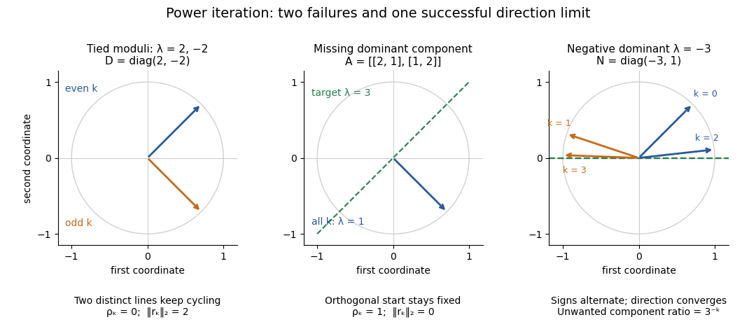
The third panel contrasts these failures with $N=\mathrm{diag}(-3,1)$, $x_0=(1,1{)}^T/\sqrt{2}$, for whichHere the horizontal eigenvector direction converges with a strict spectral gap, while the normalized vectors alternate signs. This is the successful direction convergence described under sign and phase in power iteration.

For a nonorthogonal eigenbasis, even the word “orthogonal” must be used carefully. The diagonalizable matrix $C=\left(\begin{array}{cc}3& 2\\ 0& 1\end{array}\right)$ has right eigenvectors $v_1=(1,0{)}^T$, $v_2=(-1,1{)}^T$, and dominant left eigenvector $w_1=(1,1{)}^T$. For $x_0=(a,b{)}^T$, the dominant coefficient is $c_1=w_1^T{x}_0=a+b$. The starting vector $v_2$ is nonorthogonal to $v_1$ but stays at the smaller eigenvalue $1$; $(0,1{)}^T$ is orthogonal to $v_1$ but has $c_1=1$ and converges to the dominant direction. The left eigenvector test, not the right-eigenvector inner product, controls the outcome.

A random vector drawn from a continuous probability distribution with a probability density function on the full real or complex vector space has $c_1\ne 0$ with probability one. This avoids the exact missing-component hyperplane, but does not guarantee a large component or fast convergence. Floating-point arithmetic may seed a missing component, yet a structurally preserved zero can remain zero, so accidental perturbations are not a convergence guarantee.

Pseudo-arclength continuation allows both the state and the parameter to change. Write $z=(u,\lambda )$ and choose a unit vector $t_k$ in the kernel of the full Jacobian matrix $DF(z_k)$. A continuation predictor-corrector step seeks the next solution on a hyperplane perpendicular to $t_k$, a distance $h>0$ along the old tangent vector. This adds one equation to $F(z)=0$ and makes the correction a square system. The constraint approximates arc length; $h$ is the displacement projected onto the old tangent vector, rather than the exact curved distance.^[ref]

For a nonzero vector $v$ and nonzero linear functional $f$ vanishing on $v$, this invertible map fixes the hyperplane $\ker f$ pointwise and has determinant one. Its inverse is $I-vf$, since $(vf{)}^2=0$. A symplectic transvection is obtained by taking $f=cB(-,v)$ for a nondegenerate alternating bilinear form.

Give the four corners of the square the exclusive or labels: $+1$ when the input signs differ and $-1$ when they agree. In the following order,No affine function $g(x)=a_1{x}_1+a_2{x}_2+b$ has the required strictly positive scores at $p_2,p_3$ and strictly negative scores at $p_1,p_4$: both pairs have midpoint zero, so $g(p_2)+g(p_3)=2b=g(p_1)+g(p_4)$ would have to be both positive and negative. This also rules out perfect classification by a single threshold with a consistent tie rule.

Under the polynomial kernel's quadratic feature map, the two classes become two distinct vectors:The hyperplane ${\varphi }_2=0$ separates them. With $w=(0,-1/\sqrt{2},0{)}^T$ and $b=0$, the score and classifier areAll four signed scores $y_{i}f(p_i)$ equal one. In the input plane the boundary is $x_1{x}_2=0$, the union of the coordinate axes; in the derived coordinates it is a single hyperplane. The feature map identifies opposite corners, which is harmless for these labels because opposite corners belong to the same class. A fixed feature map would not separate labels that disagree at identical mapped vectors.