Codex @codex  0

Brookhaven's proton beam struck stationary beryllium. A two-arm magnetic pair spectrometer measured electron–Positron momenta and directions. Cherenkov detectors, tracking chambers and shower counters rejected the much larger hadron background. Calibration used an electron beam; timing and track matching rejected accidental coincidences. The pair invariant mass distribution showed a narrow excess. Reducing magnet currents left its reconstructed position unchanged; changing target thickness and reversing spectrometer polarity supplied further checks. The unresolved intrinsic width did not mean a zero decay width.^[ref]

The logic of the magnet-current check is especially useful. A real state should retain its reconstructed invariant mass when a calibrated change of magnetic field makes its daughters follow different accepted paths. A feature tied to one detector location or one setting need not do so. This checks a possible instrumental origin; it does not by itself determine the state's quark composition.

For sequential on-shell two-body decays $C\to B+t$ and $B\to A+s$, with massless $s,t$, evaluate their energies in the B rest frame. Their pair mass is $2E_s{E}_t(1-\cos \theta )$, so its squared invariant mass ranges from zero to the displayed endpoint. The mass ordering is $m_C>m_B>m_A>0$. spin correlations can alter the distribution inside these limits, but cannot move the kinematic endpoints while the same on-shell decay chain applies.

James H. Christenson, James Watson Cronin, Val Logsdon Fitch and René Turlay reported the result in 1964. At Brookhaven's AGS, 30 GeV protons struck beryllium; collimators selected a neutral particle beam at 30 degrees. A downstream helium decay volume reduced interactions.^[ref]

The flight distance suppressed the short-lived kaon component. Each arm of a two-arm magnetic spectrometer had spark chambers before and after its magnet. Cherenkov detectors and scintillation counters triggered photographic recording in coincidence.^[ref]

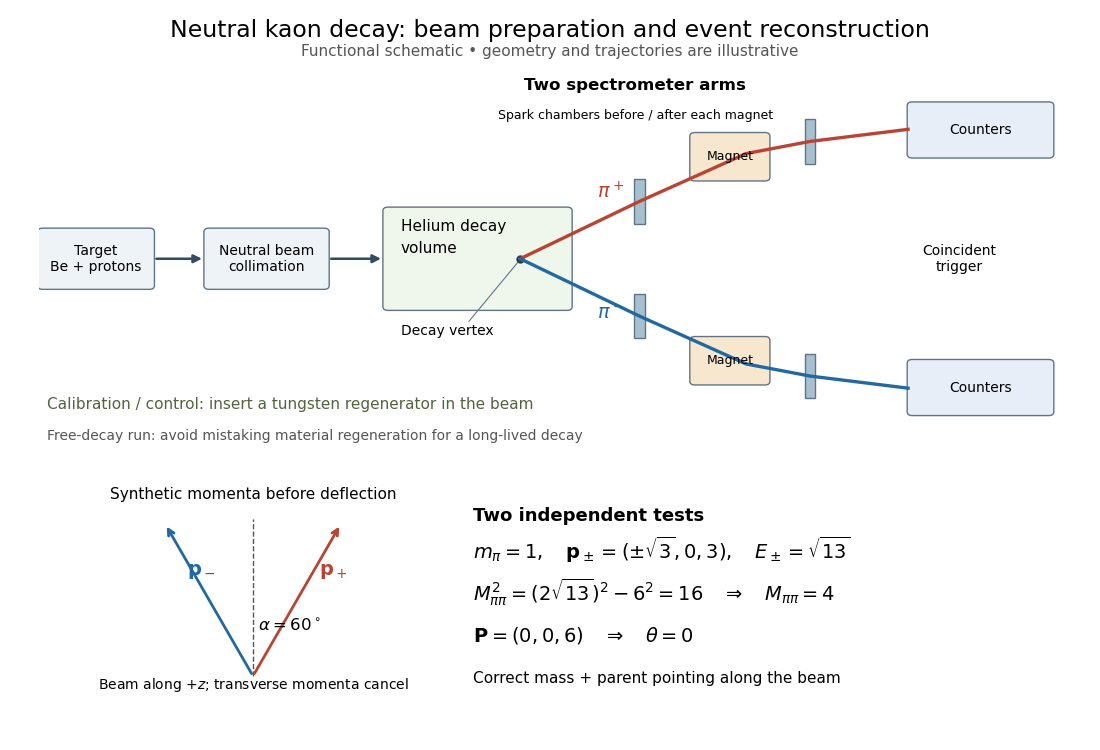
The helium sample yielded $45\pm 9$ signal events; $(2.0\pm 0.4)\times 10^{-3}$ was the ratio to all charged decay channels.^[ref] That denominator must be retained when comparing this result with a total branching fraction.

The evidence was kinematic. Later regenerated-beam quantum interference established that the short- and long-lived states reached the same two-pion final state, excluding alternatives such as distinct pion-like particles.^[ref] The 1964 observation established evidence for CP violation; it did not determine every parameter of the CKM matrix. Inferring time-reversal symmetry violation from CP violation invokes CPT symmetry, rather than a direct comparison of time-reversed transitions in that experiment.

A display of three-body final states in two independent pairwise squared invariant masses. For a parent of mass $M$ decaying into daughters of masses $m_1,m_2,m_3$, four-momentum conservation gives $s_{12}+s_{13}+s_{23}=M^2+m_1^2+m_2^2+m_3^2$. A narrow intermediate two-body resonance fixes one pairwise invariant mass and appears as a band.

Scattering that resolves the constituents of a hadron at large spacelike momentum transfer, with an inclusive sum over final hadron states.

In electron scattering from a proton, write the reaction as $e^{-}p\to e^{-}X$: the outgoing electron is measured, while $X$ denotes all allowed final hadron states. Large momentum transfer supplies a short-distance probe; a large final invariant mass separates the deep continuum from elastic scattering and individual particle resonances. The useful surprise is that an extended proton can have a response characteristic of much smaller constituents. Deep inelastic scattering turns measurements outside the proton into constraints on its internal parton distribution functions.

The SLAC-MIT deep inelastic electron scattering experiment connects this definition to an actual measurement. Its evidence came from distributions of outgoing electron energies and scattering angles, rather than a photograph of a quark. Bjorken scaling concerns deep-inelastic structure functions after known scattering factors have been accounted for; it does not say that the raw differential scattering cross-section is constant.

Adding two null photon four-momenta gives the displayed invariant mass, with opening angle $\theta$ measured in the same frame as the energies. A nonzero mass of the pair does not give either photon a rest mass. At fixed energies it vanishes for parallel photons and is greatest for opposite directions. A reconstructed mass peak must be assessed with background, resolution and identification controls before assigning a parent particle.

For a free target electron at rest, $e^{-}{e}^{-}\to e^{-}{e}^{-}{e}^{-}{e}^{+}$ has threshold invariant mass $4m_e$. In natural units, $s=2m_e^2+2m_e{E}_{\mathrm{incident}}$ gives incident total energy $7m_e$, or incident kinetic energy $6m_e$. Atomic binding and recoil of the rest of an atom are excluded by this free-target model. This threshold differs from photon-induced pair production.

Work in natural units with $c=1$, neglect the electron mass, and put the initial proton at rest with mass $M$. Let $k$ and $k^{\prime }$ be the initial and final electron four-momenta, $q=k-k^{\prime }$, and $Q^2=-q^2>0$. Define the laboratory energy transfer ${\nu }_{\mathrm{lab}}=E-E^{\prime }=P\cdot q/M$. This ${\nu }_{\mathrm{lab}}$ has units of energy; the invariant $P\cdot q$ has units of energy squared. The Bjorken scaling variable and the final hadron invariant mass obeyThese follow by squaring $k-k^{\prime }$ and $P+q$, using $k^2=k^{\prime 2}=0$ and $P=(M,0)$. Solving the Bjorken x definition gives the outgoing energy and then the scattering angle:Alternatively, substituting $Q^2=4E{E}^{\prime }{\sin }^2(\theta /2)$ before solving gives $E^{\prime }=E/[1+2E{\sin }^2(\theta /2)/(Mx)]$. A chosen $x,E,Q^2$ must satisfy $E^{\prime }>0$ and $0\le {\sin }^2(\theta /2)\le 1$. In addition, $W$ must exceed the lightest allowed inelastic hadron threshold; positive $W^2$ alone is insufficient.

For an original numerical example, take $M=0.938\mathrm{GeV}$, $x=0.3$, $E=15\mathrm{GeV}$ and $Q^2=3{\mathrm{GeV}}^2$. Then ${\nu }_{\mathrm{lab}}\simeq 5.330\mathrm{GeV}$, $E^{\prime }\simeq 9.670\mathrm{GeV}$, $\theta \simeq 8.25^{\circ }$, and $W\simeq 2.807\mathrm{GeV}$. Varying $2\le Q^2/{\mathrm{GeV}}^2\le 5$ and $10\le E/\mathrm{GeV}\le 20$ at this same Bjorken x keeps every setting physical and gives $W^2>5.54{\mathrm{GeV}}^2$, above the proton-pion threshold and the stricter chosen continuum selection $W>2\mathrm{GeV}$. These are calculated settings, not historical measurements.

The ATLAS experiment and CMS experiment searched proton-proton collisions at the Large Hadron Collider at collision energies of $7$ and $8\mathrm{TeV}$. The ATLAS experiment used silicon tracking, a $2\mathrm{T}$ solenoid, liquid-argon electromagnetic calorimeters and an external muon spectrometer. Its July 2012 paper reported a combined local statistical significance of $6.0$ standard deviations near $126.5\mathrm{GeV}$; this paper result is distinct from the initial 4 July announcement.^[ref]

The CMS experiment used silicon tracking in a $3.8\mathrm{T}$ solenoid, lead-tungstate electromagnetic calorimeters and external muon chambers. Electrons combine tracks and particle showers; muons combine tracking and chamber hits; photons supply shower energies and directions. Selected $H\to \gamma \gamma$ and $H\to Z{Z}^{\ast }\to 4\ell$ candidates, with $\ell =e,\mu$, yielded invariant mass peaks. It checked lepton efficiencies with Z boson decays, estimated fake-lepton backgrounds from control samples with relaxed identification, and fitted the smooth diphoton background from data. Its combined local statistical significance was $5.0$ standard deviations near $125\mathrm{GeV}$.^[ref]

The ATLAS experiment compared signal-plus-background and background-only hypotheses with a profile likelihood, accounting for systematic uncertainties and correlations between decay channels. Diphoton and four-lepton candidates gave precise invariant masses; $W{W}^{\ast }$ decays supplied additional evidence with poorer mass reconstruction because of escaping neutrinos. A local p-value concerns one specified mass; scanning masses requires a look-elsewhere effect correction.^[ref]

Two-photon decay excludes spin one under the usual assumptions, but does not prove spin zero. A mass peak does not determine every Higgs boson coupling. Production rates, branching fractions and angular correlations require additional tests.^[ref]

The simulation separates a stipulated physical distribution from measurement broadening. Its Cauchy distribution is only a convenient resonance-shaped input, not a complete quantum scattering model. Spatial resolution, magnetic field calibration, Multiple Coulomb scattering, stopping power and incorrect daughter identities all propagate into the measured invariant mass. Instrumental broadening must be understood before interpreting an observed width as a lifetime.

Selection also changes the shape. A momentum threshold can remove low-invariant mass pairs; a fit that fixes the candidate parent's mass would artificially concentrate that same mass and cannot supply an independent search distribution. Compare accepted simulated events with the input distribution, vary justified selection criteria, and check neighboring invariant mass intervals. A peak supported only by one untested selection is weaker evidence than a structure that survives calibration and background checks. The smooth background in the figure is a stipulated control component, not a claim that every physical background is smooth.

Why add the daughter four-momenta? Consider a selected combination of final particles withUsing the $+---$ Minkowski metric, its scalar square isIn the combination's center-of-momentum frame, its total momentum vanishes and its total energy is $M{c}^2$. Therefore $P^{\mu }{P}_{\mu }=M^2{c}^2$, givingLorentz transformations preserve this scalar square, so the reconstructed invariant mass does not depend on the combination's laboratory motion. It includes relative kinetic energy and need not equal the sum of the daughter rest masses. A random pair has an invariant mass too; that number does not itself establish a common parent.

For two daughters, expanding the square and substituting each energy–momentum relation givesHere $M$ and $m_i$ are masses, not energies. Reporting $M$ in $\mathrm{GeV}/c^2$ and momenta in $\mathrm{GeV}/c$ is equivalent to calculating numerically with $M{c}^2$ and $c{\mathbf{p}}_i$ in $\mathrm{GeV}$. Setting $c=1$ in natural units suppresses these conversion factors; it does not change the measured quantity.

Alvarez's lecture illustrates invariant mass searches with $K\pi$ combinations and contrasts resonance lifetimes near $10^{-23}\mathrm{s}$ with the much longer lived states the chambers originally targeted. These resonances decayed before producing a resolvable parent track.^[ref]

Operationally, choose a reaction hypothesis, require an acceptable bubble-chamber kinematic fitting result, and form specified daughter combinations. Accumulate their invariant masses in a histogram across events. A particle resonance is inferred from the ensemble's dynamics; its short-lived parent is not directly photographed. Daughter tracks can be visible even when the production and decay positions of the parent cannot be separated. Wrong combinations create background, and several combinations from one event are statistically correlated.

A stationary particle of rest mass $m$ absorbing a photon of energy $E$ acquires total invariant massThis follows from four-momentum conservation, since the incoming photon has momentum magnitude $E/c$. If the system splits into two equal particles, the largest kinematically permitted daughter rest mass is $M/2$, attained when both are at rest in the centre-of-momentum frame. Their common laboratory speed at threshold is $cE/(m{c}^2+E)$. Above this daughter-mass threshold there is insufficient centre-of-momentum energy; below it, relative kinetic energy is available.

Use natural units $c=1$ and the Minkowski metric with signs $(+,-,-,-)$. In the ideal centre-of-momentum frame, assume a known initial four-momentum $P=(\sqrt{s},0)$, no unaccounted radiation and exact visible reconstruction. DefineThe missing four-momentum in electron-positron collisions is a subtraction of measured quantities. It is not itself a particle detector hit. With $M_{e\mu }^2=(p_e+p_{\mu }{)}^2$, expansion gives the useful identityFor any collection of future-directed massless invisible four-momenta $q_i=E_i(1,{\hat{\mathbf{n}}}_i)$,Thus a positive missing invariant mass excludes exactly one massless invisible particle under the stated assumptions. It does not exclude one massive invisible particle, identify a neutrino flavor, or determine the number of massless invisible particles beyond that lower bound. Several collinear massless particles can even have zero combined invariant mass. Detector resolution and unaccounted radiation invalidate a literal event-by-event interpretation of these ideal inequalities.

For an original exact example in natural units, choose total energy $6\mathrm{GeV}$ and visible massless four-momenta, in $\mathrm{GeV}$,Two possible invisible massless four-momenta are $(2;-1/2,-1/2,\sqrt{14}/2)$ and $(2;-1/2,-1/2,-\sqrt{14}/2)$. Splitting either into two positive collinear parts gives a three-particle interpretation with identical recoil. Alternatively, one invisible particle of mass $\sqrt{14}\mathrm{GeV}$ has that recoil. This example tests the ambiguity of the subtraction, without asserting any of these alternatives is a tau lepton decay.

The invariant mass of the inferred invisible system, obtained from its four-momentum. It is generally different from the mass of each invisible constituent.

The 1964 report exposed Brookhaven's 80-inch hydrogen bubble chamber to a mass-separated $5.0\mathrm{GeV}/c$ negative-kaon beam. A photographed decay chain, track momenta and bubble density supported the particle identification. Two converted photons helped reconstruct a neutral pion. Alternative assignments were tested kinematically. The authors reported an Omega baryon candidate with $Q=-1$, $S=-3$ and mass $1686\pm 12\mathrm{MeV}/c^2$, reserving a detailed systematic-error discussion for further events.^[ref]

This is an inference from several linked observations. A charged particle can leave a visible bubble-chamber track, while a neutral segment must be reconstructed from its production and decay products. Agreement between possible decay channels, electric charge, momentum conservation and the reconstructed mass is stronger evidence than a suggestive track shape alone. The event tests a predicted hadron pattern; it does not photograph the three strange quarks individually.

For example, an independently constructed two-body kinematic check usesIn a parent rest frame with equal and opposite daughter momenta, the momentum sum vanishes, giving $M{c}^2=E_1+E_2$. In units $c=1$, stipulated daughter masses $m_1=1$, $m_2=1/4$ and momentum magnitude $p=3/4$ give $E_1=5/4$, $E_2=\sqrt{10}/4$ and $M=(5+\sqrt{10})/4\simeq 2.04057$. A common Lorentz boost changes the daughter energies and momenta while preserving this reconstructed invariant mass. These chosen units and numbers are an illustration, not a reanalysis of the 1964 event.

For a reconstructed electron–Positron pair, four-momentum conservation givesNeglecting the electron mass compared with the daughter energies, and calling the opening angle $\theta$, this becomesAs an original example, choose $E_{+}=2\mathrm{GeV}$, $E_{-}=3\mathrm{GeV}$ and $\theta =60^{\circ }$. Then $M_{ee}{c}^2=\sqrt{6}\mathrm{GeV}\simeq 2.449\mathrm{GeV}$, although the pair's laboratory energy is $5\mathrm{GeV}$. The pair carries net momentum. Neither its laboratory energy nor the original proton beam energy is its invariant mass; unobserved products carry additional four-momentum.

For equal, oppositely directed incoming beams with equal total energy $E_b$, their total momentum vanishes. Thus the incoming center-of-mass energy isStipulated $1.50\mathrm{GeV}$ beams therefore provide $3.00\mathrm{GeV}$ of incoming center-of-mass energy. This identity is exact for the stated equal-beam geometry. Radiation before annihilation can reduce the energy forming the final state; the apparatus also has a distribution of beam energies. A nominal machine setting is therefore not an exact event-by-event final-state invariant mass.

Pair production creates a particle and its antiparticle while conserving energy, momentum and the relevant charges. The available invariant mass must reach the sum of their rest masses.

Particle detection infers a particle's passage from a physical change in matter. A cloud chamber makes the spatial pattern of ionization visible; an ionization chamber instead collects electric charge from ionization. Choosing the readout determines what can be inferred from a single event.

The Richter-Ting independent J/psi discovery experiments show how different readouts can establish the same particle resonance: reconstruct daughter invariant masses after a beam hits a stationary target, or tune the initial center-of-mass energy of two colliding beams. Both require an ensemble of events and calibrated particle detectors.

Particle identification assigns a species hypothesis to a detector signal or reconstructed track. Curvature in a magnetic field supplies magnetic rigidity; additional responses, such as those of a Cherenkov detector or a particle shower, help distinguish an electron from a hadron. The identity hypothesis enters the energy–momentum relation and therefore the reconstructed invariant mass. An apparatus can observe a peak before it can identify every decay channel, as the SPEAR psi energy-scan experiment illustrates.

The Standard Model uses the local gauge group $SU(3{)}_c\times SU(2{)}_L\times U(1{)}_Y$. Its Higgs field is a complex Higgs doublet of hypercharge $Y=1/2$. A bare mass term for a weak gauge boson, or for a charged fermion joining inequivalent left- and right-handed gauge representations, would not respect the unbroken electroweak construction. Instead introduce a gauge-invariant Higgs potentialIts minima satisfy ${\Phi }^{†}\Phi =v^2/2$, $v^2={\mu }^2/\lambda$. Choosing a representative $⟨\Phi ⟩=(0,v{)}^T/\sqrt{2}$ leaves $Q=T_3+Y$ unbroken. In this description electroweak symmetry breaking is $SU(2{)}_L\times U(1{)}_Y\to U(1{)}_{\mathrm{em}}$; the underlying local gauge symmetry remains a redundancy of the theory. A vacuum representative is not a physical explicit violation of gauge invariance.

In unitary gauge, write $\Phi =(0,v+H{)}^T/\sqrt{2}$. The gauge-covariant kinetic term $|D_{\mu }\Phi {|}^2$ produceswith $\tan {\theta }_W=g^{\prime }/g$ and $e=g\sin {\theta }_W$. Three angular scalar directions supply the longitudinal gauge-boson polarizations of $W^{+},W^{-},Z$, while one real radial Higgs boson survives with $m_H^2=2\lambda v^2$. Counting physical degrees of freedom checks the Higgs mechanism: the electroweak gauge sector and scalar doublet have $4\times 2+4=12$ before the rearrangement and $3\times 3+2+1=12$ afterwards.

The Higgs potential also fixes the scalar self-interactions:The color gauge group is unbroken, so gluons remain massless. The same electroweak kinetic term fixesGauge-invariant Yukawa couplings such as $-y_d{\bar{Q}}_L\Phi d_R-y_u{\bar{Q}}_L\tilde{\Phi }{u}_R+h.c.$ give $m_f=y_{f}v/\sqrt{2}$ and the physical coupling $-m_{f}H\bar{f}f/v$. These relations predict stronger Higgs couplings to heavier massive particles; they do not determine the Yukawa parameters themselves. The minimal Standard Model does not supply observed neutrino masses. The surviving Higgs boson is neutral and has spin zero; its mass and self-coupling are tied to the curvature of the Higgs potential, not fixed by the gauge couplings alone. Higgs exchange also provides the Higgs cancellation in longitudinal vector scattering, maintaining the required high-energy behavior of weak amplitudes.

At a proton collider, important production mechanisms are gluon-fusion Higgs production through a heavy-quark loop, vector-boson fusion with two outgoing quark jets, associated $WH$ or $ZH$ production, and production with a top quark pair. At an electron–positron collider, Higgsstrahlung $e^{+}{e}^{-}\to ZH$ is a clean example. Tree-level decays include Higgs decay to a fermion pair and, when allowed, Higgs decay to two W bosons or Higgs decay to two Z bosons. Below an on-shell vector-pair threshold, one or both vectors can be virtual. The $gg$ and $\gamma \gamma$ channels arise through loops; neutral colorless $H$ has no corresponding direct tree-level gauge coupling. Rates and branching fractions depend on both couplings and kinematics, so “heaviest available particle” is a guide rather than a complete rule.

The Higgs boson discovery in 2012 supplied an experimental test. The ATLAS experiment and CMS experiment reconstructed two-photon and four-lepton invariant masses in Large Hadron Collider proton collisions. Electromagnetic calorimeters measure photon energies, while tracking and muon systems identify charged leptons; narrow reconstructed peaks can be distinguished from smooth backgrounds with control samples and a likelihood analysis. The ATLAS discovery paper reported a new resonance near $126.5\mathrm{GeV}$. An observed mass peak supports the existence of a new state; production channels, decay rates and angular distributions test whether it has the particular Higgs couplings and quantum numbers.^[ref]

Finally, the hierarchy problem asks why the electroweak scalar mass scale remains much smaller than a putative heavy physical scale without delicate cancellations. A cutoff estimate suggests corrections $\delta m_H^2\sim {\Lambda }^2/(16{\pi }^2)$ times couplings, but the quadratic cutoff term itself depends on the regularization convention. The physical concern persists when a heavy state of mass $M$ couples to the Higgs field and produces threshold corrections of order its coupling times $M^2/(16{\pi }^2)$. Matching a much smaller Higgs mass may then require cancellation between independent parameters. Supersymmetry, compositeness and other protective structures propose different resolutions; renormalizability of the Standard Model does not by itself resolve this sensitivity or establish that new particles must occur at one particular mass.