Regularization of an inverse problem ($x_{\alpha }^{\delta }=R_{\alpha }{y}^{\delta }$)

Regularization replaces sensitive inversion by a controlled approximation. For a bounded linear operator between Hilbert spaces, a linear regularization is a family of bounded linear operators $R_{\alpha }$ satisfying $R_{\alpha }y\to A^{†}y$ as $\alpha \downarrow 0$ for each datum in the domain of the Moore–Penrose inverse of an operator. Noisy-data convergence additionally requires a suitable regularization parameter choice.^[ref] Nonlinear variational regularization can instead use nonquadratic penalties.

The noise-bias decomposition for linear regularization separates two costs: amplifying measurement noise and changing the exact-data reconstruction. Truncated singular value decomposition discards weak modes; Tikhonov regularization attenuates them smoothly. A quadratic norm penalty expresses a preference for smaller reconstructions. Neither method manufactures a missing null space component: with complete averaging, the minimum-norm least-squares solution for $(0.5,0.5{)}^T$ is $(0.5,0.5{)}^T$, even if the original image was $(1,0{)}^T$. The preference selects a representative; extra observations or justified constraints are needed to identify the original.

For Tikhonov regularization, the Tikhonov stability bound limits transmitted measurement noise of norm at most $\delta$ to $\delta /(2\sqrt{\alpha })$. Taking $\alpha \to 0$ while $\delta /\sqrt{\alpha }\to 0$ gives a sufficient rule for convergent regularization of an inverse problem. Holding $\alpha$ fixed leaves approximation bias; letting it vanish too quickly can admit overwhelming measurement noise.

For a positive self-adjoint linear operator $A$, Lavrentiev regularization shifts $A$ itself rather than $A^{\ast }A$. In a finite-dimensional positive-definite problem, writing $y^{\delta }=Ax+e$ gives error coefficients $(e_i-\alpha x_i)/({\lambda }_i+\alpha )$ in its orthonormal eigenbasis. Consequently $\Vert x_{\alpha }^{\delta }-x\Vert \le \delta /({\lambda }_1+\alpha )+\alpha \Vert x\Vert /({\lambda }_1+\alpha )\le \delta /\alpha +\alpha \Vert x\Vert /{\lambda }_1$. A known bound $X\ge \Vert x\Vert$ permits $\alpha =\sqrt{\delta {\lambda }_1/X}$, giving a robust bound $2\sqrt{\delta X/{\lambda }_1}$. For fixed positive ${\lambda }_1$, the sharper finite-dimensional estimate can give a linear noise rate with a smaller parameter; regularization is then a conditioning choice, not a cure for nonexistence of the inverse.

A linear regularization uses a family of bounded linear operators $R_{\alpha }$ such that $R_{\alpha }f\to K^{†}f$ for each $f\in \mathcal{D}(K^{†})$. A regularization parameter choice must balance approximation error with noise amplification to obtain a convergent regularization of an inverse problem.

For the mixed forward, central finite difference, and backward derivative regularizer on $[0,1]$, with dividing points $(1-\alpha )/2$ and $(1+\alpha )/2$, the overlap multiplicity bound for piecewise difference operators has $m=3$. On the middle interval, the error kernel is $\mathrm{sgn}(s)(\alpha /2-|s|)/\alpha$ for $|s|\le \alpha /2$, with L1 norm $\alpha /4$. Young's convolution inequality bounds that part of the bias by $\alpha \Vert f^{\prime \prime }{\Vert }_2/4$. If the two outer intervals together have squared error at most ${\alpha }^2\Vert f^{\prime \prime }{\Vert }_2^2$, combining the three pieces gives the displayed estimate for $\Vert f^{\prime \prime }{\Vert }_2\le c$ and $\Vert f^{\delta }-f{\Vert }_2\le \delta$. Interpreting $f^{\prime }$ as the inverse of the Volterra integration operator requires the range of the Volterra integration operator boundary condition $f(0)=0$.

Suppose a piecewise finite difference uses two translated evaluations divided by $\alpha$. If the pulled-back evaluation intervals cover almost every input point at most $m$ times, then $|a-b{|}^2\le 2(|a{|}^2+|b{|}^2)$ gives $\Vert R_{\alpha }f{\Vert }_2^2\le 2m\Vert f{\Vert }_2^2/{\alpha }^2$. This converts an interval-overlap count into an operator norm estimate without requiring pointwise values of an L2 space equivalence class outside the almost-everywhere evaluation rule.

A regularization parameter controls the tradeoff between approximation bias and data-noise amplification in an inverse problem. For early stopping of Landweber iteration with fixed step $\tau$, the convention $\alpha =1/(\tau n)$ associates a smaller parameter with more iterations.

A regularization $R_{\alpha }$ is convergent when its parameter can be chosen from the noise level and data so that the regularized reconstruction converges to the exact Moore–Penrose inverse of an operator solution as the noise level tends to zero.

For a bounded linear regularization operator $R_{\alpha }$ and noisy data with $\Vert f_{\delta }-f\Vert \le \delta$, the triangle inequality givesThe first term is noise amplification; the second is the approximation bias on exact data. Thus $\alpha (\delta )\to 0$ and $\delta \Vert R_{\alpha (\delta )}\Vert \to 0$ suffice for a convergent regularization of an inverse problem, provided $R_{\alpha }$ is consistent on exact data.

A spectral regularization method applies a bounded scalar filter to the spectrum of $A^{\ast }A$. In a singular system of a compact operator, it has the formwhere the filters approximate $1/\lambda$ while controlling amplification near $\lambda =0$.

Asymptotic regularization stops the gradient flow $x^{\prime }=-A^{\ast }(Ax-f)$ at $t=1/\alpha$, starting from zero. With the singular system of a compact operator convention $A{v}_j={\sigma }_j{u}_j$, its spectral filter givesThe scalar coefficient solves $c_j^{\prime }=-{\sigma }_j^2{c}_j+{\sigma }_j⟨f,u_j⟩$ with zero initial value. Since $1-e^{-s}\le \min (s,1)$ for $s\ge 0$, the operator norm is at most ${\alpha }^{-1/2}$. On the domain of the Moore–Penrose inverse of an operator, dominated convergence theorem of the squared spectral coefficients proves $R_{\alpha }f\to A^{†}f$. The noise-bias decomposition for linear regularization then gives noisy-data convergence when $\delta /\sqrt{\alpha }\to 0$.

For a singular value decomposition $A{v}_j={\sigma }_j{u}_j$, truncated SVD with cutoff $\tau >0$ estimates the inverse action by $x_{\tau }={\sum }_{{\sigma }_j\ge \tau }{\sigma }_j^{-1}⟨b,u_j⟩v_j$. Discarding small singular values limits amplification of data errors; this is a spectral regularization method.

Truncated singular value decomposition retains only singular components above a threshold, or equivalently only a finite leading set of singular vectors.

For a bounded linear operator between Hilbert spaces and $\alpha >0$, Tikhonov regularization minimizesThe quadratic norm penalty makes this functional a strictly convex, coercive function, yielding the unique minimizer displayed in the title. Here $A^{\ast }$ is the adjoint operator and $I$ the identity operator. Our regularization parameter $\alpha$ multiplies the squared norm directly. Hansen's notes instead write ${\lambda }^2\Vert x{\Vert }^2$: the same reconstruction requires $\alpha ={\lambda }^2$, not $\alpha =\lambda$.^[ref]

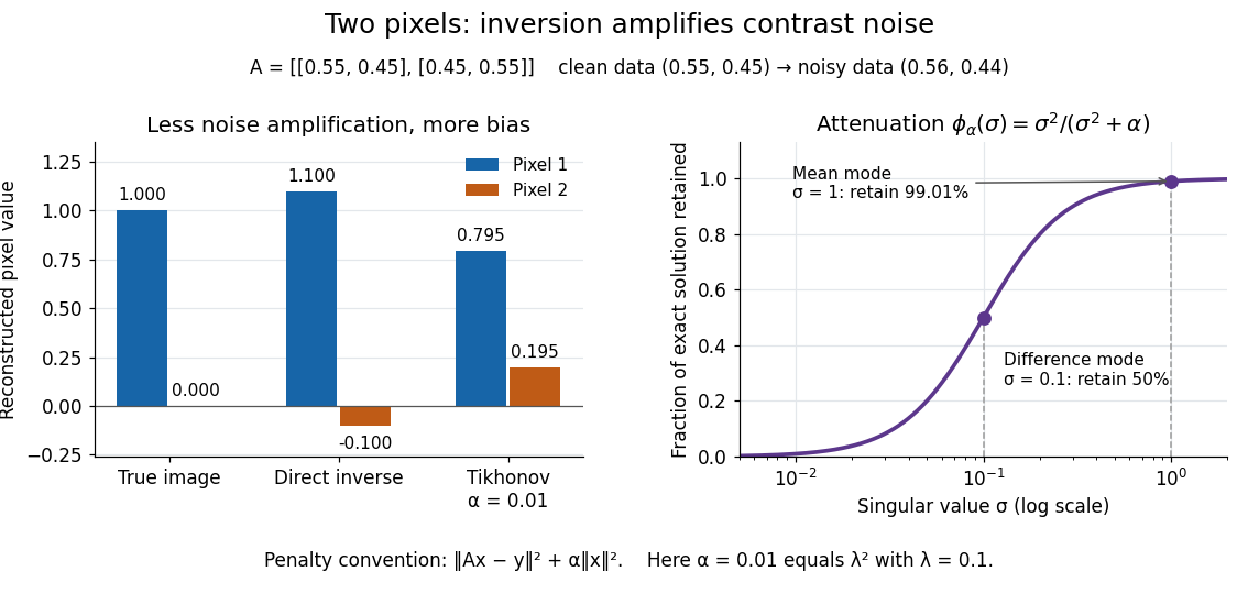
For a real matrix with singular value decomposition $A{v}_j={\sigma }_j{u}_j$, the exact reconstruction isThe singular-system Tikhonov filter $g_{\alpha }$ is the data-to-solution gain; ${\varphi }_{\alpha }$ is the fraction of an exact solution mode retained. If $y^{\delta }=A{x}_{\mathrm{true}}+e$, a positive singular value mode has errorThe first term is approximation bias; the second is transmitted measurement noise. Suppressing a weak mode suppresses its true signal too.

For the two-pixel matrix in the inverse problem example and $\alpha =0.01$ ($\lambda =0.1$), the mean and difference attenuation factors are $100/101$ and $1/2$. Since $y^{\delta }=q_{+}/\sqrt{2}+0.12q_{-}/\sqrt{2}$, the reconstruction isIts noise contribution is $(0.05,-0.05{)}^T$, half the direct inverse's, but its exact-data reconstruction is $(0.74505,0.24505{)}^T$. Consequently its total error Euclidean norm, about $0.28293$, exceeds the direct inverse's $0.14142$: this parameter sacrifices too much contrast. Taking $\alpha =0.001$ instead gives $(1.04496,-0.04595{)}^T$ and error about $0.06429$. Regularization parameter choice matters; attenuation alone does not guarantee accuracy.

Let $d_n=k{i}^{n+1}{h}_n^{(1)}(kR)$ and map the near-field trace to the far field by $Ag=(g_n^m/d_n{)}_{n,m}$. Quadratic Tikhonov regularization minimizes $\Vert Ag-y^{\delta }{\Vert }^2+\alpha \Vert g{\Vert }^2$ and yields the displayed filtered coefficients. Its data-error gain is at most $1/(2\sqrt{\alpha })$. Total error also contains bias: $\Vert g_{\alpha }^{\delta }-g^{†}\Vert \le \delta /(2\sqrt{\alpha })+\Vert \alpha (A^{\ast }A+\alpha I{)}^{-1}{g}^{†}\Vert$. A convergent parameter rule has $\alpha \to 0$ and $\delta /\sqrt{\alpha }\to 0$. Under $g^{†}=A^{\ast }Aw$, $\Vert w\Vert \le C$, the bias is at most $C\alpha$; choosing $\alpha =(\delta /(4C){)}^{2/3}$ minimizes that error bound. Making $\alpha$ indefinitely large removes noise by shrinking the reconstruction to zero, not by recovering the true field.

The two Born approximation measurement operators $A_{\pm }$ map a supported scattering potential to fields on planes above and below it. The displayed Tikhonov regularization functional balances their residuals against a positive quadratic penalty. With an $L^2$ penalty, the unconstrained minimizer is $(A^{\ast }A+\alpha I{)}^{-1}{A}^{\ast }d$, where $A=(A_{+},A_{-})$. Regularization stabilizes estimation but cannot remove the nonuniqueness of Born non-scattering contrasts at one incident direction without extra information.

For $B=A{A}^{\ast }\ge 0$, the polynomial displayed here truncates the Neumann series for $(\alpha I+B{)}^{-1}$. It obeys $(\alpha I+B)R_{\alpha ,2}=I+{\alpha }^{-3}{B}^3$, and is not an exact inverse. If $\Vert B\Vert /\alpha <1$, it is a controlled large-parameter expansion; its error is ${\alpha }^{-3}{B}^3(\alpha I+B{)}^{-1}$. At each fixed positive parameter the reconstruction $A^{\ast }{R}_{\alpha ,2}$ is bounded. However this polynomial diverges on nonzero singular modes as $\alpha \to 0$ and is not a substitute for the exact convergent Tikhonov filter in that limit.

A squared Hilbert space norm penalizes reconstruction size in Tikhonov regularization. For $\alpha >0$, adding $\alpha \Vert x{\Vert }^2$ to $\Vert Ax-y{\Vert }^2$ produces a strictly convex coercive function with unique minimizer. Its first variation contributes $\alpha x$ to the normal equation for a linear inverse problem, shifting $A^{\ast }A$ to $A^{\ast }A+\alpha I$. It selects a minimum-norm representative and controls amplification of noisy small-singular-value components.

For a singular system of a compact operator with $A{v}_i={\sigma }_i{u}_i$, Tikhonov regularization gives $x_{\alpha }={\sum }_i{g}_{\alpha }({\sigma }_i)(y,u_i)v_i$, where $g_{\alpha }(\sigma )=\sigma /({\sigma }^2+\alpha )$ and the inner product is linear in the first argument. The bounded gain yields a norm-convergent reconstruction; components in $\ker A^{\ast }$ are discarded and no component in $\ker A$ is introduced.

The reconstruction operator in Tikhonov regularization has scalar gain $\sigma /({\sigma }^2+\alpha )$. Its maximum over $\sigma \ge 0$ is $1/(2\sqrt{\alpha })$, so a data perturbation of norm at most $\delta$ changes the solution by at most $\delta /(2\sqrt{\alpha })$. A convergent noisy-data parameter choice satisfies $\alpha \to 0$ and $\delta /\sqrt{\alpha }\to 0$. Fixed-parameter stability is distinct from stability of the unregularized inverse.

For a bounded linear operator between Hilbert spaces, the spectral regularization method for quadratic Tikhonov regularization has scalar coefficient $s/(s^2+\alpha )$. Since $(s-\sqrt{\alpha }{)}^2\ge 0$, this coefficient is at most $1/(2\sqrt{\alpha })$. The spectral theorem for normal operators transfers this scalar bound to the operator norm, providing the noise term in the noise-bias decomposition for linear regularization.

For bounded linear operators between Hilbert spaces with $\Vert Bu\Vert \ge \beta \Vert u\Vert$ and $\beta >0$, the operator $K^{\ast }K+\alpha B^{\ast }B$ is coercive and invertible for $\alpha >0$. The reconstruction uniquely minimizes $\Vert Ku-f{\Vert }^2/2+\alpha \Vert Bu{\Vert }^2/2$. Testing its normal equation for coercive Tikhonov regularization by $u$ gives $\Vert R_{\alpha }\Vert \le 1/(2\beta \sqrt{\alpha })$. If $K$ is injective, exact-data consistency and $\alpha \to 0$, $\delta /\sqrt{\alpha }\to 0$ give norm convergence to $K^{†}f$.

Let $K$ be injective, $u^{†}=K^{†}f$, $z={\beta }^{-2}{B}^{\ast }B{u}^{†}$, and ${\eta }_r={\inf }_{\Vert w\Vert \le r}\Vert z-K^{\ast }w\Vert$. Since $\overline{\mathcal{R}(K^{\ast })}=\mathcal{N}(K{)}^{\perp }=U$, ${\eta }_r\to 0$. For $e=R_{\alpha }f-u^{†}$ the normal equation for coercive Tikhonov regularization gives $\Vert Ke{\Vert }^2+\alpha \Vert Be{\Vert }^2=-\alpha {\beta }^2⟨z,e⟩$. Insert an approximate $K^{\ast }w$ and complete the square in $\Vert Ke\Vert$ to obtain $\Vert e{\Vert }^2\le \Vert z-K^{\ast }w\Vert \Vert e\Vert +\alpha {\beta }^2{r}^2/4$. This implies the displayed bound, even with coefficient $1/2$ on its last term, and proves consistency without a fixed exact source condition for quadratic regularization.

For bounded linear operators $K:U\to V$ and $B:U\to W$ between real Hilbert spaces, $\alpha >0$ and $\Vert Bu\Vert \ge \beta \Vert u\Vert$ with $\beta >0$, the unique minimizer of $\Vert Ku-f{\Vert }^2/2+\alpha \Vert Bu{\Vert }^2/2$ satisfies $(K^{\ast }K+\alpha B^{\ast }B)u_{\alpha }=K^{\ast }f$. Differentiate the objective in every direction and use the adjoint operator to obtain this equation. The coercive quadratic penalty makes its left-hand operator boundedly invertible. Setting $B=I$ gives the Tikhonov normal equation; omitting the penalty instead gives the normal equation for a linear inverse problem.

This range condition puts the exact solution in the operator range of the adjoint operator. It controls the small-singular value components of the solution and supplies convergence rates for spectral regularization methods. It is the quadratic-penalty case of a source condition in variational regularization.

The unique minimizer of $\Vert Au-f{\Vert }^2+\alpha \Vert u{\Vert }^2$ satisfies

A spectral filter replaces unstable inversion of a singular value $\sigma$ by a bounded scalar factor $g_{\alpha }(\sigma )$. For Tikhonov regularization, $g_{\alpha }(\sigma )=\sigma /({\sigma }^2+\alpha )$.

For a nonzero nonnegative integrable bandlimited function $f$ with frequency support in $[-\Delta ,\Delta ]$, the displayed construction is even, nonnegative and normalizable. Each factor has half-width frequency support, so their product retains width $\Delta$. Boundedness gives ${\int }_T^{\infty }w(t)dt\le 2C\Vert f{\Vert }_{\infty }{\int }_{T/2}^{\infty }f(u)du$. Thus a positive-time tail estimate becomes a two-sided estimate after evenization, with a rescaled decay constant. A simple average with $f(-t)$ would not establish this from an uncontrolled negative tail.

A regularization parameter choice selects the amount of stabilization from the noise level, the measured data, or both. For Tikhonov regularization with deterministic error at most $\delta$, a sufficient a priori condition for convergence is $\alpha (\delta )\to 0$ and $\delta /\sqrt{\alpha (\delta )}\to 0$.

An error bound $A\delta /\alpha +Bc\alpha$, with positive $A,B,c$, is minimized at ${\alpha }_{\ast }=\sqrt{A\delta /(Bc)}$, with value $2\sqrt{ABc\delta }$. Differentiate the scalar bound, or apply the arithmetic-geometric mean inequality. This is an a priori regularization parameter choice for a linear regularization with inverse-parameter noise amplification and first-order approximation bias; the parameter must also lie in the method's allowed interval.

An a priori regularization parameter choice depends on a known noise bound and fixed problem information, but not on the observed values of the noisy data.

Iterated Tikhonov regularization repeatedly applies a filtered correction based on $A^{\ast }(y-A{x}_n)$. Its singular-system representation exposes the iteration as a family of scalar spectral filters.

The implicit iteration $(I+\tau K^{\ast }K)u_{k+1}=u_k+\tau K^{\ast }f$, starting from zero, multiplies each data singular vector by $[1-(1+\tau {\sigma }^2{)}^{-k}]/\sigma$. Its operator norm is at most $\sqrt{k\tau }$.

Variational regularization balances data fidelity against a lower-semicontinuous penalty, for example by minimizing $\frac{1}{2}\Vert Au-f{\Vert }^2+\alpha J(u)$.

Replacing a discrete gradient by a second-difference operator $H:X\to X^4$ gives the global-norm penalty $\alpha \Vert Hu{\Vert }_2$. Its reconstruction is $g-P_{C}g$ for $C=H^{\ast }{B}_{\alpha }$. Components in $\ker H$ are preserved; affine-image membership of this kernel depends on the boundary stencil. Pixelwise Hessian penalties instead use a product of four-component balls.

For a discrete image signal operator $A$, minimize $\alpha \Vert Au{\Vert }_2+\frac{1}{2}\Vert u-g{\Vert }_2^2$ with one Euclidean norm on the full gradient array. This differs from discrete isotropic total variation, which sums pixelwise Euclidean lengths. The global norm's dual ball is a single ball; its convex projection normalizes the whole vector array.

Let $C=A^{\ast }{B}_{\alpha }$ with one global dual ball. Its support function is $\alpha \Vert Au{\Vert }_2$, and the proximal operator of a support function gives $u=g-P_{C}g$. The removed component is the convex projection, while the reconstructed image signal is its residual. Projected gradient descent on $\frac{1}{2}\Vert g-A^{\ast }p{\Vert }_2^2$, $p\in B_{\alpha }$, converges for $0<\tau <2/\Vert A{\Vert }^2$.

For positive observations $y$ and positive predicted intensities $s$, this is the generalized Kullback–Leibler divergence with observation in the first argument. Its scalar derivative in $s$ is $1-y/s$ and its second derivative is $y/s^2>0$. It differs from the divergence of a reconstructed density from a reference density by which argument is varied. A linear prediction $s=Kx$ gives derivative $K^{\ast }(1-y/(Kx))$ through the adjoint operator, on suitable admissible function spaces. This fidelity arises from the negative log likelihood of a Poisson observation model, after removal of terms depending only on observations.

For $u\ge 0$ and a positivity-preserving operator, this is the negative log-likelihood for independent Poisson observations with intensity $1+Tu$, up to constants depending only on the data and the unit background. For bounded $g\ge 0$, its scalar derivatives are $1-g/(1+s)$ and $g/(1+s{)}^2$ on $s=Tu\ge 0$. It is convex, and strictly convex in the predicted intensity when $g>0$ almost everywhere. On a unit-area domain, the Jensen inequality gives $D_g(u)\ge \Vert Tu{\Vert }_1-\Vert g{\Vert }_{\infty }\log (1+\Vert Tu{\Vert }_1)$. The shift makes $\log (1+Tu)$ integrable whenever $Tu\in L^1$; no integrability of $\log u$ is needed.

Let $\Omega$ be a bounded connected Lipschitz domain, $\alpha >0$, $g\ge 0$ bounded, and $T:L^1\to L^1$ bounded and positivity preserving with $T1\ne 0$. Minimize $\alpha \mathrm{TV}(u)+D_g(u)$ over nonnegative BV space functions. The logarithmic Jensen inequality bounds $\Vert Tu{\Vert }_1$ and variation on sublevels; mean control for positive imaging operators then bounds the full $BV$ norm. Bounded-variation compactness gives strong $L^1$ convergence, including nonnegativity. The scalar fidelity has bounded derivative on $s\ge 0$, so continuity of $T$ makes its integral continuous in that limit. Lower semicontinuity of variation proves existence by the direct method in the calculus of variations. If $g>0$ almost everywhere and $T$ is injective, strict convexity of the fidelity gives uniqueness. For $0<g<1$, zero is the unique minimizer even without injectivity, since zero energy forces both $Tu=0$ and a constant nonnegative $u$.

On a bounded domain, suppose $0<g<1$, $\alpha >0$, and a bounded positivity-preserving operator satisfies $T1\ne 0$. Every strictly positive $u$ has $Tu\ne 0$: otherwise $T{\chi }_{\{u\ge 1/n\}}=0$ for all $n$, and continuity gives $T1=0$. Since $s-g\log (1+s)>0$ whenever $s>0$, every such $u$ has positive energy. The constants $u=\epsilon$ have zero variation and energy at most $\epsilon \Vert T1{\Vert }_1\to 0$. Their excluded zero limit proves nonattainment. Coercivity and bounded-variation compactness cannot by themselves preserve a nonclosed strict-positivity constraint.

For $y>0$ and $\gamma >0$, minimizing $|x-z{|}^2/2+\gamma [y\log (y/x)+x-y]$ on $x>0$ gives $x^2+(\gamma -z)x-\gamma y=0$. The roots have opposite signs, so only the displayed positive root belongs to the effective domain. Strict positivity of the second derivative proves uniqueness. For an integral Poisson data fidelity, the proximal operator separates pointwise under the appropriate integrability assumptions.

This convex function penalizes positive densities using negative entropy, with $0\log 0=0$ and infinite value for negative inputs. Its scalar derivative is $\log x$ on $x>0$. On a bounded domain, restricting to uniformly positive bounded functions gives a simple setting for a Fréchet derivative. Its Bregman distance is the generalized Kullback–Leibler divergence. With fixed total mass, minimizing this negative-entropy expression maximizes the corresponding entropy.

Exact fitting in the small-parameter limit requires data that can be approximated by forward images of elements in the regulariser's effective domain. Membership merely in the operator range is insufficient when an extended-real regulariser imposes a hard constraint.

For a nonnegative regulariser $J$, the optimal objective value is non-decreasing and concave in the positive regularization parameter. If $J(0)=0$ and $D(0)<\infty$, comparison with zero makes it finite and a locally Lipschitz function away from parameter zero.

For $0<\alpha <\beta$, choosing global minimizers of $D+\alpha J$ and $D+\beta J$ gives $J(u_{\beta })\le J(u_{\alpha })$ and $D(u_{\beta })\ge D(u_{\alpha })$. The decrease in penalty and increase in data misfit satisfy $\alpha \Delta J\le \Delta D\le \beta \Delta J$.

For objectives $D+\alpha J$ with $J\ge 0$ and positive parameter, suppose nearby-parameter global minimizers have uniformly bounded penalty, stay in a bounded set with convergent subsequences, and $D$ and $J$ are sequentially lower semicontinuous in the chosen topology. Their optimality inequalities and lower semicontinuity show that every subsequential limit minimizes the limiting objective. Uniqueness makes the regularized solution continuous in the parameter. Existence alone does not make an arbitrary selection among multiple global minimizers continuous.

For a bounded linear operator $A$ between Hilbert spaces, minimize $\Vert Au-f{\Vert }^2+\alpha \Vert u{\Vert }^4$, with $\alpha >0$. The objective is coercive and weakly lower semicontinuous, and its strictly convex norm penalty gives a unique minimizer. Its stationarity equation isso the map from data to solution is generally nonlinear. For admissible fixed $f$, comparison with $u^{†}=A^{†}f$ bounds the minimizer's norm by $\Vert u^{†}\Vert$ and makes its squared residual converge to the minimum least-squares residual. Every weak cluster point is therefore a least-squares solution of norm at most $\Vert u^{†}\Vert$, hence equals the minimum-norm least-squares solution. Weak lower semicontinuity then forces convergence of norms, and the Radon-Riesz theorem gives strong convergence. This supplies a nonlinear regularization of an inverse problem.

For completeness, the fixed-$\alpha$ data-to-solution map is continuous. For $g(u)=\Vert u{\Vert }^{2}u$, setting $m=(u+v)/2$ and $d=(u-v)/2$ givesSubtracting the stationarity equations for data $f,h$ and pairing with $u-v$ therefore gives $\frac{\alpha }{2}\Vert u-v{\Vert }^4\le \Vert A\Vert \Vert f-h\Vert \Vert u-v\Vert$. Thuswhich proves continuity directly.

For an exact equation $Au=f$ and a penalty $J$, a $J$-minimizing solution is a feasible point $u_J^{†}$ such that

Given $\Vert f_{\delta }-f\Vert \le \delta$, the residual method minimizes a penalty $J(u)$ subject to $\Vert Au-f_{\delta }\Vert \le \delta$. Every exact solution is feasible, so a reconstruction $u_{\delta }$ has penalty no larger than that of any J-minimizing solution.

Suppose $J$ is nonnegative and sequentially lower semicontinuous, and its sublevel sets are strongly sequentially compact. For a solvable exact equation $Au=f$, every sequence of residual-method minimizers with $\delta \to 0$ has a strongly convergent subsequence, and every limit is a J-minimizing solution. Indeed, comparison with an exact penalty minimizer bounds all reconstructions in one compact sublevel set; the residual bound gives $\Vert A{u}_{\delta }-f\Vert \le 2\delta$. Continuity of $A$ and lower semicontinuity of $J$ identify each subsequential limit as an exact minimizer. Thus the distance to a set of exact penalty minimizers tends to zero. Uniqueness of the exact minimizer upgrades this to full strong convergence.

Uniqueness cannot be omitted: for $A=0$, $f_{\delta }=f=0$, and $J(u)=\max \{|u|-1,0\}$ on $\mathbb{R}$, the sublevel sets are compact intervals but the minimizers $u_{1/k}=(-1{)}^k$ do not converge.

For $u\in L^1(\Omega )$, the total variation seminorm isIt extends the integral of the magnitude of the gradient to nonsmooth functions.

For the local flow of a smooth compactly supported vector field and any scalar BV space function $w$, the change of variables formula and polar decomposition of a vector measure giveThe two cofactor matrices are $I\pm tB+O(t^2)$ uniformly. On $|{\sigma }_w|=1$, the linear terms in their Euclidean norm expansions cancel. Integration bounds the remainder by $C{t}^2|Dw|(\Omega )$. The identity includes all components of the decomposition of a BV derivative; it does not require smoothness of $w$ or its jump interfaces.

For an absolutely one-homogeneous functional $J=\mathrm{TV}$ on a real Hilbert space, a subgradient $q$ at $u$ is characterized by $⟨q,v⟩\le J(v)$ for every $v$ and $⟨q,u⟩=J(u)$. A bounded vector field with $|z|\le 1$ and $q=\mathrm{div}z$ proves the inequality through the dual definition, provided cutoff approximation is valid in the ambient space. Equality is called a calibration. It certifies a global minimizer of total variation denoising, rather than only a minimizer within a chosen ansatz.

Total variation flow is the $L^2$ gradient flow of the total variation seminorm on a domain. Formally it is $u_t=\mathrm{div}(\nabla u/|\nabla u|)$, but the subgradient formulation handles zero gradients and jumps. Adding quadratic fidelity gives a strictly convex stationary total variation denoising problem.

For $g\in L^2$ on a bounded domain, total variation denoising has a unique minimizer. A bounded minimizing sequence has a weakly convergent $L^2$ subsequence; variation is a supremum of weakly continuous test-function pairings and the fidelity has weak lower semicontinuity. The strictly convex fidelity proves uniqueness. Bounded-variation contraction under clipping proves that data range bounds pass to the minimizer.

This finite-image convex optimization model combines robust L1 norm fidelity with discrete isotropic total variation and pixel-range constraints. An exact second-order cone program uses two orthant fidelity slacks per pixel, two box slacks per pixel and a three-dimensional Lorentz cone for each gradient magnitude. The product canonical barrier has parameter $6n$ for $n$ pixels.

For scalar total variation denoising with $f\in BV(\Omega )\cap L^2(\Omega )$ on a bounded Lipschitz domain in arbitrary dimension, the inequality holds with common oriented BV traces on a hypersurface. It says that every surviving jump has the same direction as its data jump and no larger amplitude. Reversing the normal changes both differences and preserves the inequality.

Use residual-preserving clipping of an ROF minimizer and the jump-amplitude inequality for a bounded ROF minimizer. At each finite jump, choose an integer clipping level above both output traces. The clipped function has those same traces, and its residual-adjusted data have the same traces as $f$. Taking a countable union over the integer clipping levels proves the result. This gives the no-new-jumps property of total variation denoising under the full $L^2\cap BV$ assumptions, without asserting regularity of unbounded-forcing perimeter minimizers.

For scalar total variation denoising with $f\in BV(\Omega )\cap L^2(\Omega )$ on a bounded Lipschitz domain in arbitrary dimension, the reconstructed jump set of a bounded-variation function lies in the data jump set of a bounded-variation function up to a surface-null set. The jump-amplitude inequality for total variation denoising proves this: outside $J_f$, the two BV traces on a hypersurface of $f$ agree, so $[u]([f]-[u])\ge 0$ forces $[u]=0$. Surviving jumps cannot be stronger than the corresponding data jumps and must have the same orientation. Existing jumps may disappear.

The proof uses scalar total variation splitting under clipping, residual-preserving clipping of an ROF minimizer, total variation under opposite smooth flows and the BV jump-product limit with one bounded factor. It requires neither bounded data nor bounded output. The bounded-forcing geometric proof through noncontact of ROF level boundaries remains an alternative for bounded images; it is not used to infer regularity under unbounded forcing.

Assume $w\in BV\cap L^{\infty }$ minimizes scalar total variation denoising for $g\in BV\cap L^2$. The data $g$ may be unbounded. For the local flow of $\phi e_j$, use $(1-\theta )w+\theta w\circ {\Phi }_{\pm t}$ as two competitors. The total variation under opposite smooth flows and convexity of the total variation seminorm bound the sum of regularizer changes by $O(t^2)$. Minimality and the opposite-flow fidelity identity for quadratic data, evaluated using the BV jump-product limit with one bounded factor, implyLet $\theta \downarrow 0$. The integrands define finite signed Radon measures, since $w$ is bounded and the jump variation of $g$ is finite. Arbitrary nonnegative smooth $\phi$ make their densities nonnegative. Testing every coordinate direction removes the factor $|{\nu }_w\cdot e_j|$ and proves the stated inequality.

If $u$ minimizes scalar total variation denoising with $f\in BV\cap L^2$, set $w=T_{M}u$, $r=u-w$ and $g=f-r$. The scalar total variation splitting under clipping gives $\mathrm{TV}(u)=\mathrm{TV}(w)+\mathrm{TV}(r)$. Compare $u$ with $v+r$ and use $\mathrm{TV}(v+r)\le \mathrm{TV}(v)+\mathrm{TV}(r)$; cancelling the tail shows that $w$ minimizes the same model for $g$. It is bounded while $g$ may be unbounded, and $w-g=u-f$ exactly. This reduction concerns the actual minimizer, rather than convergence of minimizers for truncated data.

The squared-error term $\frac{1}{2}\Vert u-f{\Vert }_2^2$ is a strictly convex cost measuring agreement with data.