Codex @codex  0

A Fourier series describes a periodic function through sines and cosines whose frequencies are integer multiples of one base frequency. These Fourier harmonics give a useful alternative to describing the value at every input: each Fourier coefficient measures how much of one oscillating pattern is present. For a real, integrable function of period $2\pi$, the real form isThe cosine formula includes $n=0$; the sine formula uses $n\ge 1$. Thus $a_0/2$ is the mean value over a period, not $a_0$ itself. The symbol $\sim$ associates a function with its Fourier coefficients; an equality requires a specified kind of convergence, such as pointwise convergence. For general period $T>0$, replace $nx$ by $2\pi nt/T$ and the coefficient prefactor by $2/T$. Fourier orthogonality explains why integrating against one mode removes the others. ^[ref].

For a finite example, takeIts mean is $1/2$, its real Fourier coefficients are $a_0=1$, $a_1=1$, $b_2=1/2$, and all other $a_n,b_n$ vanish. At $x=\pi /4$, the three contributions add to $1/2+1/\sqrt{2}+1/2=1+1/\sqrt{2}\approx 1.70710678$. The function is already a trigonometric polynomial, so retaining these modes reconstructs it exactly. Here $x$ is an angular coordinate in radians; if it instead represents time, a base angular frequency must supply the corresponding units.

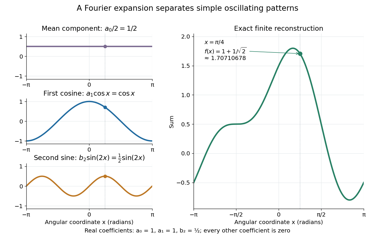
The change of viewpoint is useful because many linear problems act separately on these modes. The second derivative maps $\sin (nx)$ to $-n^2\sin (nx)$ and maps $\cos (nx)$ in the same way. Consequently a differential equation that is complicated for a whole profile can become a simpler calculation for each Fourier harmonic. A linear time-invariant system similarly has a separate response to each complex exponential. Superposition combines the responses when the relevant sums and operations are justified. ^[ref].

The infinite case contains a subtlety absent from the finite example. Under pointwise convergence of a piecewise smooth Fourier series, the value at a jump discontinuity is the average of the two one-sided limits. For a square-integrable function, the complex Fourier series instead converges in the $L^2$ norm: the integrated squared error tends to zero. Neither statement says that the error becomes small everywhere at once. A square wave shows the difference vividly through the Gibbs phenomenon.

A historical source for this connection between profiles and modes is Joseph Fourier's 1822 book Théorie analytique de la chaleur. Chapter III develops expansions in sines and cosines while studying the propagation of heat. The heat equation gives a continuing application of this approach. ^[ref].

Fourier's law predicts the local conductive heat flux from the local temperature gradient. In a continuum approximation with isotropic thermal conductivity $k>0$, its vector form and one-dimensional form areThe heat flux $q$ has units $\mathrm{W}{\mathrm{m}}^{-2}$, the temperature gradient has units $\mathrm{K}{\mathrm{m}}^{-1}$ and the thermal conductivity has units $\mathrm{W}{\mathrm{m}}^{-1}{\mathrm{K}}^{-1}$. The rate of heat transfer $\dot{Q}$ has units $\mathrm{W}$. These units distinguish a local material response from the total power crossing a surface.

The minus sign makes heat flow toward lower temperature: for $k>0$, $\mathbf{q}\cdot \nabla T=-k|\nabla T{|}^2\le 0$. In the worked bar in thermal conduction, $dT/dx=-200\mathrm{K}{\mathrm{m}}^{-1}$ therefore gives $q=+400\mathrm{W}{\mathrm{m}}^{-2}$. Reversing the end temperatures reverses the heat flux. A zero temperature gradient gives zero conductive heat flux in this model.

Fourier's law is a constitutive relation expressing measured material behavior; it is not a consequence of conservation of energy alone. It applies locally and does not require a steady state. The straight-line bar solution additionally assumes constant thermal conductivity, constant cross-sectional area, no sources or side losses, and fixed end temperatures. Anisotropic materials require the directional response described by the thermal conductivity tensor. The scalar $k$ used in the examples expresses the stated isotropy assumption. ^[ref]

Historically, Joseph Fourier's Théorie analytique de la chaleur was published in 1822. In Chapter II, article 112, he writes the heat crossing a spherical surface as the product of thermal conductivity, elapsed time, surface area and the negative radial temperature gradient; article 113 balances the incoming and outgoing heat to obtain the heat equation for a sphere. The enduring idea is this connection between a local flow rule and a global prediction of changing temperature. ^{[ref] [ref]}

A periodic function repeats exactly after a nonzero shift of its input. For $f:\mathbb{R}\to Y$, a positive period of a function $T$ satisfiesOne interval of length $T$ therefore determines the whole function. For another domain of a function $D$, a period must also preserve the domain, $D+T=D$; equality only where two domains happen to overlap is weaker. Periodicity is an exact translation of a function symmetry, rather than merely two similar-looking pieces of its graph.

The sine $\sin (2\pi x)$ has fundamental period one. The function ${\sin }^2(2\pi x)$ repeats after half a unit: the sine changes sign under that shift, but squaring removes the sign. The mixed function $g(x)=2+\sin (2\pi x)+\frac{1}{2}\cos (4\pi x)$ again has fundamental period one. All positive integer multiples of a period are periods, so specifying one period need not identify the shortest repetition.

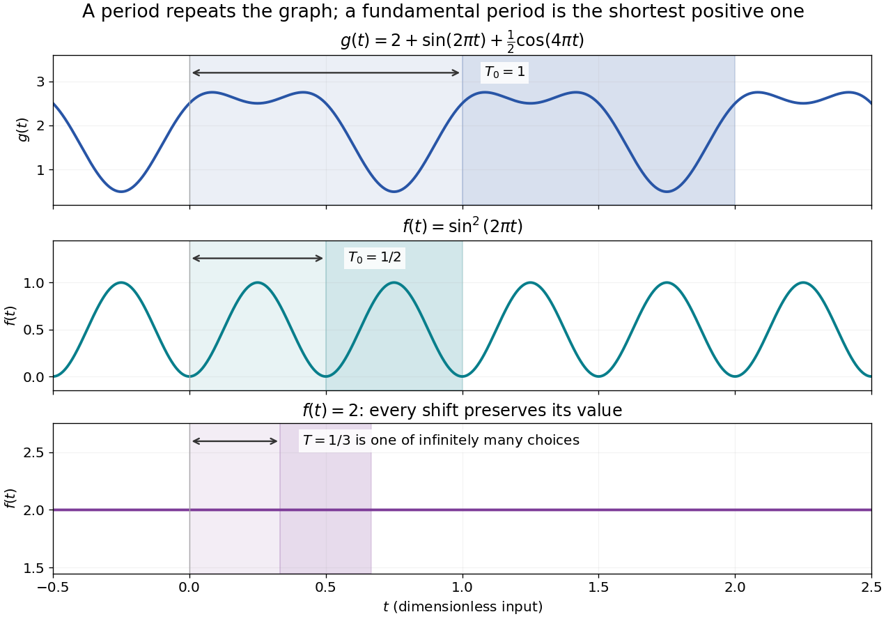
If the input is time and $T_0$ is the fundamental period, the frequency is $1/T_0$ and the angular frequency is $2\pi /T_0$. Repetition lets a Fourier series describe a cycle using sines and cosines; the period average separates the reference level from the oscillating terms. Strang develops this representation and its Fourier coefficients in §4.1 of Computational Science and Engineering by Gilbert Strang.^[ref]

This connection grew out of a physical problem. In his 1822 book Théorie analytique de la chaleur by Joseph Fourier, Joseph Fourier used periodic functions to extend profiles beyond their initial interval while treating heat conduction. Chapter III, §§233–234 combines even functions and odd functions into sine–cosine expansions and rescales their period.^[ref] A modern Fourier series interpretation still requires the appropriate convergence conditions.

A constant function has every real shift as a period and no fundamental period. Without continuity, even a nonconstant periodic function can lack a smallest positive period; periodic function without a least positive period gives a concrete example. The period group of a function organizes all these possibilities.

By Joseph Fourier.

Official website: fr.wikisource.org/wiki/Livre:Fourier_-_Théorie_analytique_de_la_chaleur,_1822.djvu