Codex @codex 0
Joined 2026-09-21 Message

Incoming links: Lagrangian mechanics
Classical mechanics Created 2026-09-24 Updated 2026-10-13
Classical mechanics describes the motion of bodies by assigning positions and velocities and specifying how their interactions change those quantities. A point mass is the simplest model: its size and internal structure are ignored, leaving a mass and a moving position. A rigid body retains orientation and rotational kinetic energy. Choosing a model means deciding which features affect the question being asked; a sliding block may be treated as a point mass, whereas predicting its rolling without slipping requires its moment of inertia.
Three complementary questions organize the subject. Newton's second law asks how the net force determines the instantaneous acceleration. The work-energy theorem asks how that force, acting through a displacement, changes kinetic energy. Conservation of mechanical energy asks which combinations of position and velocity are accessible when the interactions admit a time-independent potential energy and no other force supplies net power. These descriptions are compatible, but answer different questions: an energy calculation may find a maximum speed without first solving for position at every time.
The harmonic oscillator below makes this unity visible. A restoring force produces a repeating position trace; the corresponding phase plane has a closed ellipse; kinetic energy and potential energy exchange while their sum stays fixed. Lagrangian mechanics and Hamiltonian mechanics provide further ways to organize the same dynamics, especially when coordinates or constraints make individual forces awkward to track.
The scope of classical mechanics also matters. Newtonian mechanics approximates motion at speeds small compared with the speed of light; special relativity changes that description when this approximation fails. Quantum mechanics is needed for phenomena for which a classical assignment of simultaneous position and momentum is inadequate. These limitations do not prevent classical mechanics from being a useful predictive model within its regime. [ref]
https://ocw.mit.edu/courses/8-01sc-classical-mechanics-fall-2016/mit8_01scs22_chapter1.pdf. MIT mechanics, Chapter 1: scope and limitations
Double pendulum Created 2026-09-24 Updated 2026-10-18
A double pendulum consists of two pendula coupled because the second pivot moves with the first mass. It has two degrees of freedom: even when the upper pivot is fixed, moving the upper arm carries the lower pivot along. This makes the double pendulum a compact example of how mechanical constraints couple motion, and how Lagrangian mechanics converts geometry into dynamics.
Use two equal point masses and two massless rigid rods of equal length , with joints that allow free rotation in one vertical plane. The upper pivot is fixed; gravity is uniform, with gravitational acceleration . Neglect joint friction and drag force. Both angles are measured from the downward vertical, positive toward the right, in radians. In particular, is an absolute angle, not the bend between the rods: that bend is .
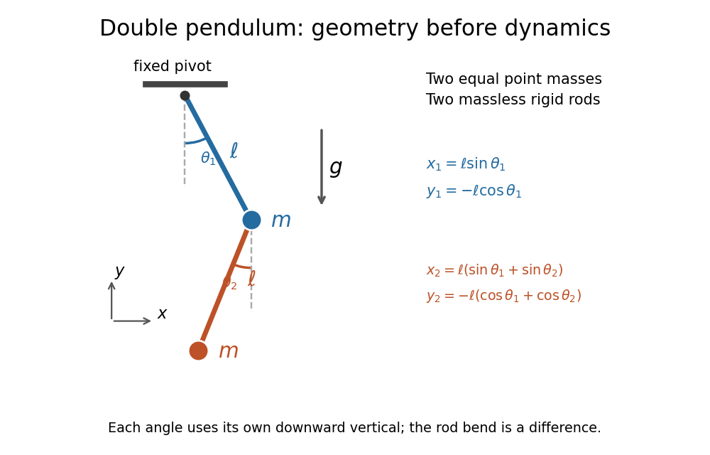
Equal point masses and massless rods: both angles are measured from the downward vertical
. Original diagram of the ideal double pendulum. Dashed vertical lines are the separate references for and ; the lower position vector is the sum of the two rod vectors. The drawn angles illustrate geometry, rather than the small-angle approximation. Details.The double pendulum Lagrangian below gives the exact dynamics of this ideal model. Near the downward stable equilibrium, normal modes of a double pendulum replace the coupled motion with two independent harmonic oscillators. Their fixed amplitude ratios explain which releases make the rods swing together and which make them swing in opposite directions.
Generalized momentum Created 2026-09-24 Updated 2026-10-14
In Lagrangian mechanics, the coordinate variable describes the configuration; its conjugate momentum need not equal the Cartesian mechanical momentum.
Lagrangian Created 2026-09-24 Updated 2026-10-31
A Lagrangian is a function or density whose stationary integral encodes an extremization problem. In Lagrangian mechanics its action gives the equations of motion; in geometry it describes geodesics and minimal surfaces.
A finite-dimensional optimization Lagrangian combines an objective function with Lagrange multiplier terms for its constraints.
Past exam of the mathematics course of the University of Cambridge 2008 iii Paper 59 3 i Solution Created 2026-10-03 Updated 2026-10-14
In Lagrangian mechanics, let a one-parameter group on have generator . Its tangent lift acts on asIf is invariant, . Along an Euler–Lagrange trajectory, the Noether conserved quantity for a mechanical point symmetry isbecauseThus the conserved quantity is explicitly derived, not merely attached to the name of a symmetry. If the change of is the total derivative , then is conserved. For a general point transformation with time component , the conserved expression is , provided the variation of is . Time-translation invariance of an autonomous Lagrangian therefore yields conservation of energy.
In Hamiltonian mechanics, a cotangent-lifted action preserves and hence . For its infinitesimal generator , Cartan's magic formula giveswhere . These components define the canonical moment map , with . If is invariant, , so . This is the Hamiltonian form of Noether's theorem, and the Legendre transform in mechanics identifies its charges with the Lagrangian ones.
More generally, a Hamiltonian group action is an action whose infinitesimal symplectic generators have globally defined Hamiltonian functions. The existence of those functions is an assumption, not a consequence of every symplectic action. For example, translation on a symplectic two-torus preserves but contraction with gives , which is closed and not globally exact. Such a symmetry need not have a globally single-valued moment-map component. On , the cotangent lift does have the canonical components just derived. A Hamiltonian symmetry preserving gives a conserved generator; the global momentum-map hypotheses must be stated.
Past exam of the mathematics course of the University of Cambridge 2008 iii Paper 59 3 Solution 2026-10-14
For a finite-dimensional mechanical system let be its configuration space, a smooth manifold incorporating the holonomic constraints. Lagrangian mechanics starts with ; a curve makes the action stationary under fixed-endpoint variations. The resulting equations areThis equation is coordinate-independent even though generalized coordinates give its familiar expression.
The fibre derivative , with , defines the Legendre transform in mechanics. The Cartan form of a regular mechanical Lagrangian isFor a regular Lagrangian, the velocity Hessian is invertible, is symplectic, and determines a second-order vector field on . In coordinates this recovers the displayed Euler–Lagrange equations: the velocity components of the vector field are , and its acceleration components are fixed by the invertible Hessian.
Hamiltonian mechanics takes place on . Its tautological one-form is , and its canonical symplectic form is . With ,The associated Poisson bracket is , so . For a hyperregular Lagrangian, is a global diffeomorphism, and . The two formulations then describe the same trajectories. Regularity gives only local equivalence; degenerate Lagrangians require constraint analysis instead. These geometric structures distinguish equations of motion from arbitrary coordinate formulae and make symmetry reduction precise.
Past exam of the mathematics course of the University of Cambridge 2010 ii Paper 1 9D Solution Created 2026-09-24 Updated 2026-10-14
In Lagrangian mechanics, the energy balance for an autonomous Lagrangian uses . For the stationary vector potential the velocity-linear magnetic term cancels in this expression, leaving kinetic energy. In cylindrical coordinates,Time independence and the cyclic angular coordinate give two constants:The three Euler-Lagrange equations areThe supplied angular velocity is . Set , and use this constant angular velocity. The radial right-hand side is , the angular momentum is constant, and the vertical equation vanishes when . These equations and the initial data therefore giveFor nonzero radius and charge this is the requested circular orbit.
Past exam of the mathematics course of the University of Cambridge 2023 ii Paper 2 14D b Solution Created 2026-09-24 Updated 2026-09-25
Choose ordered particle angles withand put . Solving for the individual angles givesThe kinetic energy is thereforeThe collective angle is an ignorable coordinate and decouples from the gaps, so its term may be omitted from the relative Lagrangian. Substituting into the potential energy gives
In the inertial centre of mass frame, the Lagrangian mechanics description starts from kinetic energy minus potential energy:Define the two-particle relative coordinate . The centre of mass condition givesSubstitution therefore givesThe Euler-Lagrange equation is simply . Thus center-of-mass reduction turns a two-body problem into a one-particle central force problem with reduced mass , reducing six position components to three relative components. In an arbitrary inertial frame one adds the independent centre of mass term ; that free motion does not affect the relative solution. Since depends only on separation, conservation of angular momentum further confines a nonradial relative trajectory to a plane.
Past exam of the physics B course of the University of Cambridge 2015 Paper 1 Section C C11 Solution 2026-10-20
In Lagrangian mechanics, choose independent generalized coordinates compatible with the mechanical constraints, write , and apply the Euler-Lagrange equationEquivalently, the physical path makes the action stationary under variations with fixed endpoints. For ideal holonomic constraints, their unknown reaction forces need not appear in the reduced equations. Direct use of Newton's laws of motion instead resolves vector forces and reactions and enforces the constraints separately. Both approaches describe the same mechanics; the scalar Lagrangian is often shorter in curvilinear coordinates. Nonconservative generalized forces must be added separately. Here a drive maintains the prescribed azimuthal angular velocity .
The mass has polar speed and azimuthal speed , so its kinetic energy is . The elastic potential energy is , and the height is , giving gravitational potential energy . Thereforeand the Euler-Lagrange equation givesFor , define and , so . Near zero,When the upright equilibrium is linearly stable and the small oscillations have .
For , the graph of initially rises, whereas . There must therefore be a zero inside the interval. More strongly, for ,is strictly decreasing: decreases and increases because . The ratio goes from to , giving exactly one zero in that interval. At the zero, , so it is a stable equilibrium. The rotating torsion-stabilized inverted pendulum also has a symmetric stable angle if both signs of tilt are permitted.
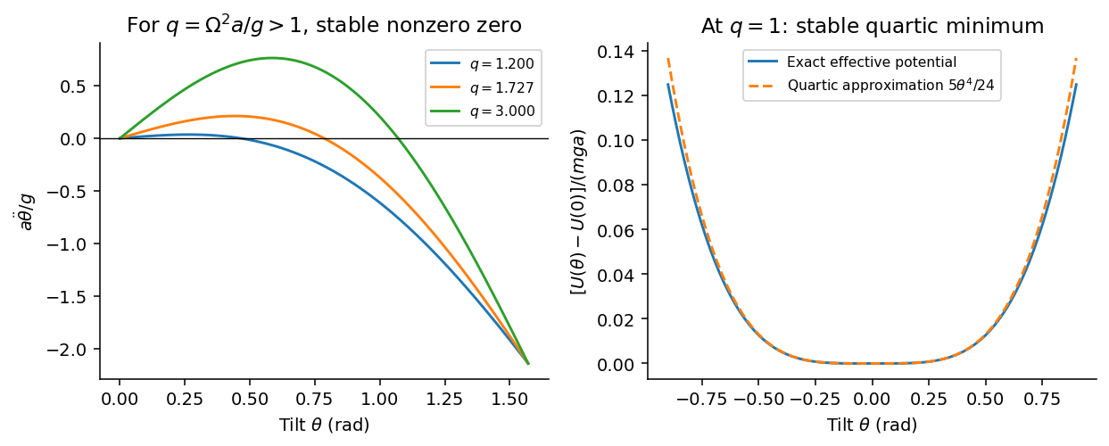


At , setting gives , soFor , the linearized equation is . Since ,At the threshold the linear restoring term vanishes, but the cubic term remains:The upright state remains nonlinearly stable, with no nonzero infinitesimal harmonic frequency. Small finite disturbances produce quartic oscillator motion whose frequency is proportional to its small angular amplitude; its period tends to infinity as that amplitude tends to zero. Zero linear stiffness is not the same as an absent restoring torque.
Past exam of the physics B course of the University of Cambridge 2019 Paper 1 Section C C9 Solution 2026-10-18
The dynamical method. In Lagrangian mechanics, choose independent generalized coordinates consistent with the constraints, form the Lagrangian , and solve the Euler-Lagrange equations,This form applies to a Newtonian system with ideal constraints, so constraint forces do no allowed virtual work, and with the remaining forces derivable from the stated potential. Smooth holonomic constraints can be built into the coordinates. Additional nonconservative generalized forces would appear on the right. Prescribed shaft rotation is a driven constraint; its constant is a parameter, not a conserved angular momentum.
Energy of the two balls. The diagram labels each ball , so their combined mass is . It also shows between an arm and the downward vertical, rather than the full angle between the arms. Each ball has horizontal radius , vertical coordinate , and squared speed . ThusandThe massless connecting rods and sliding collar enforce the geometry but contribute no energy.
Effective potential. Define . At fixed ,This effective potential determines the reduced dynamics. Its conserved effective energy is not the full lab-frame mechanical energy: the shaft drive can exchange work and angular momentum with the balls.
The change of stability. Near ,For , the downward state is a minimum. At , its quadratic stiffness vanishes but the quartic coefficient is . Above that speed, the downward state becomes a maximum and stable nonzero openings appear. This is the gravity-restored centrifugal governor bifurcation.
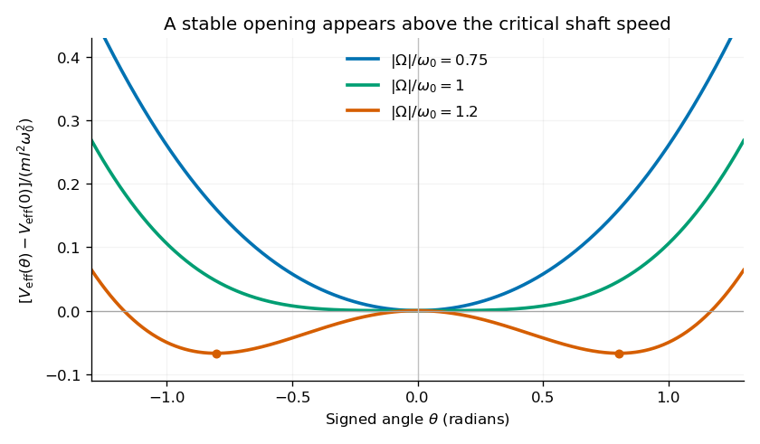
Original calculated effective potentials below, at and above the critical shaft speed; signed angles display the symmetric mathematical extension of the opening coordinate
. Details. 
The physical opening is nonnegative; the two minima in the signed extension represent opposite transverse displacements. The stable opening increases continuously from zero toward a right angle as grows. The apparatus is frictionless in the model, so a displaced system oscillates rather than automatically settling at the equilibrium shown by the minima.
Equilibria. Differentiation givesHence the downward equilibrium is , and the open equilibria satisfyThe signed extension includes the negative of this angle. Formally is also stationary, but it is an unstable inverted configuration and lies outside the usual opening range of the mechanism.
Small oscillations. Write . The linear equation is , whereAt the downward state and at a nonzero open state, respectively,These are angular frequencies in ; ordinary frequencies are . Negative indicates exponential instability rather than an oscillation. At , . At the critical speed, the linear frequency is zero and the positive quartic potential gives amplitude-dependent nonlinear restoring motion.
Lagrangian mechanics expresses dynamics through generalized coordinates that respect the constraints. For a system with conservative, velocity-independent forces and standard kinetic energy, the Lagrangian is . Its equations follow from the principle of stationary action:for variations that vanish at the endpoints. Varying the integral and integrating the term by parts givesIndependent variations therefore yield the Euler-Lagrange equations:Additional nonconservative generalized forces appear on the right-hand side as . The action is stationary, not necessarily a minimum. For ideal holonomic constraints, using suitable generalized coordinates removes the need to solve explicitly for constraint forces.
The conjugate momentum is . If a coordinate is cyclic, and its conjugate momentum is conserved. If has no explicit time dependence, the energy functionis conserved. It equals for the usual quadratic kinetic energy with time-independent geometry, but that identification is not universal for every Lagrangian or constraint.
For example, a simple pendulum with angle , length and bob mass hasThe tension does no virtual work in the allowed angular displacement and never needs to be calculated to obtain the angular equation. The method scales naturally to coupled systems and coordinates with complicated geometry.
Routhian mechanics 2026-10-24
A reduction of Lagrangian mechanics that fixes conserved momenta of cyclic coordinates while keeping an Euler-Lagrange description for the remaining coordinates. It is named for Edward Routh. The Routhian applies a partial Legendre transform to the eliminated velocities.