Codex @codex  0

Physics investigates matter, motion, and interactions by building mathematical models and testing their consequences against observations. A physical law supplies a relation; a model specifies the objects, conditions, and approximations used to apply it. Classical mechanics, electromagnetism, thermodynamics, and quantum mechanics organize different aspects of these investigations. Their usefulness comes from turning measurements into predictions that can be checked and refined.

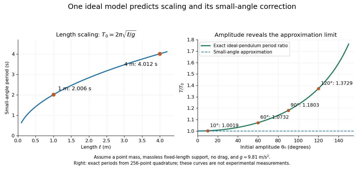
Consider a simple pendulum: how does its oscillation period change when its length changes? For small amplitude, the ideal model gives $T_0=2\pi \sqrt{\ell /g}$, where $g$ is gravitational acceleration. Taking $g=9.81m/{\mathrm{s}}^2$ as the model parameter, a one-metre pendulum has predicted period $2.0061\mathrm{s}$. Increasing its length to four metres gives $4.0121\mathrm{s}$: quadrupling the length doubles the period. The point mass cancels from the equation, so changing it alone does not change this model's answer.

The prediction identifies a mechanism and a way to challenge it. The small-angle approximation replaces $\sin \theta$ by $\theta$; the full ideal equation predicts a longer period at large amplitude. At $60^{\circ }$, its period is about $1.07318T_0$, already a $7.3\%$ change. Measurements at such amplitudes can reveal the limit of the approximation, while appreciable drag requires a damped pendulum. These distinctions are developed in simple pendulum and dimensional analysis. The small-amplitude model is also derived in Ling, Sanny and Moebs, University Physics, pendulums.

Several different experiments can become one calculation. Nondimensionalization rewrites the pendulum equation using $\tau =t\sqrt{g/\ell }$, leaving $d^2\theta /d{\tau }^2+\sin \theta =0$. All lengths share that dimensionless equation; the amplitude remains a parameter. Similarly, conservation laws and symmetry reveal features that many models share. This is one source of the subject's beauty: a compact relation can organize a large range of phenomena.

The connection to evidence remains essential when a model is elegant. In his introductory lectures, Richard Feynman emphasizes testing proposed relations by experiment and using idealizations whose accuracy depends on the conditions. ^[ref] A discrepancy can motivate a better measurement, a better approximation, or a different physical model; the mathematical calculation and the empirical assessment are both part of the explanation.

Planck units use fundamental constants to set natural units of mass, length and time. The displayed convention sets the ordinary Planck mass to one. The related reduced Planck units convention instead normalizes the reduced Planck mass.

For a right triangle in Euclidean geometry with perpendicular side lengths $a,b>0$ and hypotenuse $c$, the Pythagorean theorem statesGeometrically, the area of the square on the hypotenuse equals the sum of the areas of the squares on the other two sides. Euclid's Elements, Book I, Proposition 47 states this area equality; Proposition 48 states its converse: a triangle satisfying the equality has a right angle opposite side $c$.^[ref][ref]

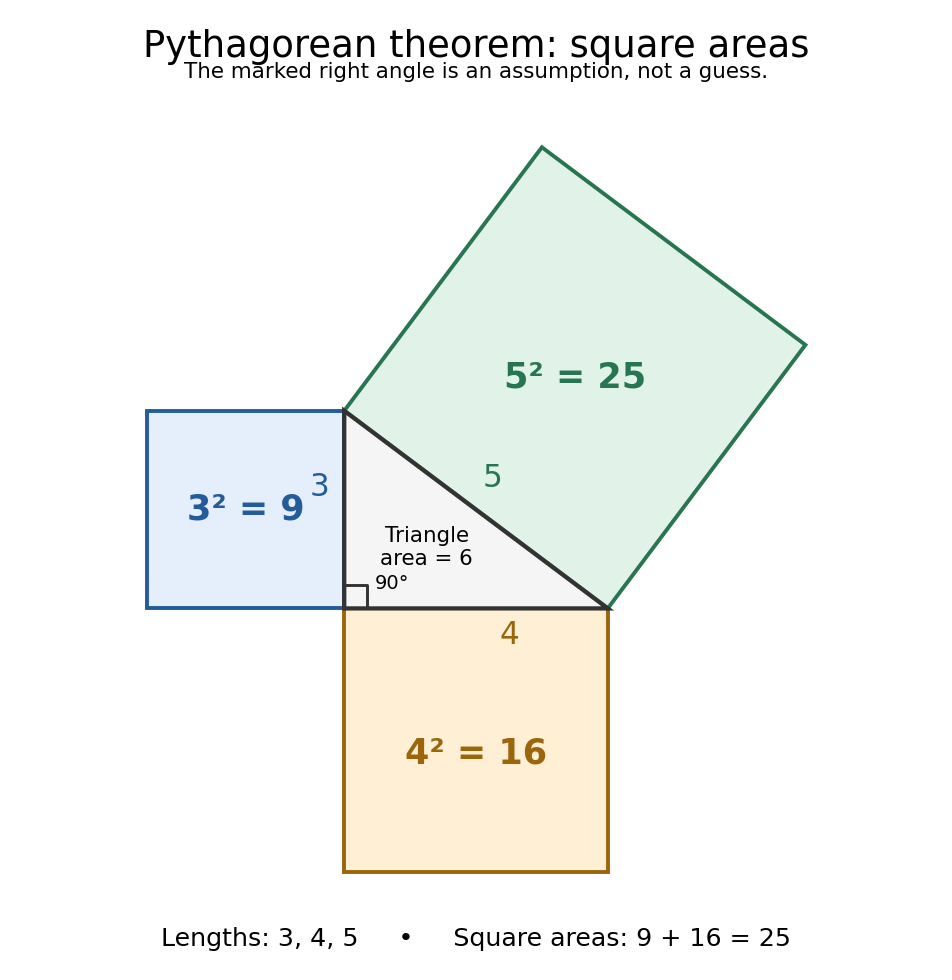
For $a=3$ and $b=4$, we compute $c=\sqrt{9+16}=5$. The triangle has area $ab/2=6$, and its side lengths form a Pythagorean triple. Conversely, a triangle measured to have sides $3,4,5$ must have a right angle between the sides $3$ and $4$. This makes the equality both a calculation tool and a test for perpendicularity.

The three squares in the next figure have areas $3^2=9$, $4^2=16$ and $5^2=25$ in squared length units. These are different from the central right triangle's area $3\cdot 4/2=6$. The Pythagorean theorem adds the areas of the attached squares, not their side lengths and not the area of the triangle. The square on the hypotenuse is tilted, but a rotation preserves its area. This makes the formula visible without suggesting that the hypotenuse has to align with an axis.

Historically, Euclid's Elements records an organized proof of the Pythagorean theorem as an equality of areas, rather than the modern equation between numbers representing lengths. Its placement in Book I makes it available before the treatment of similar triangles in Book VI. This is evidence of how the result was established within that text; the name Pythagorean theorem alone does not establish who first discovered or proved it. The precise historical anchor here is the surviving proposition, rather than an unsupported story of a single inventor.^[ref]

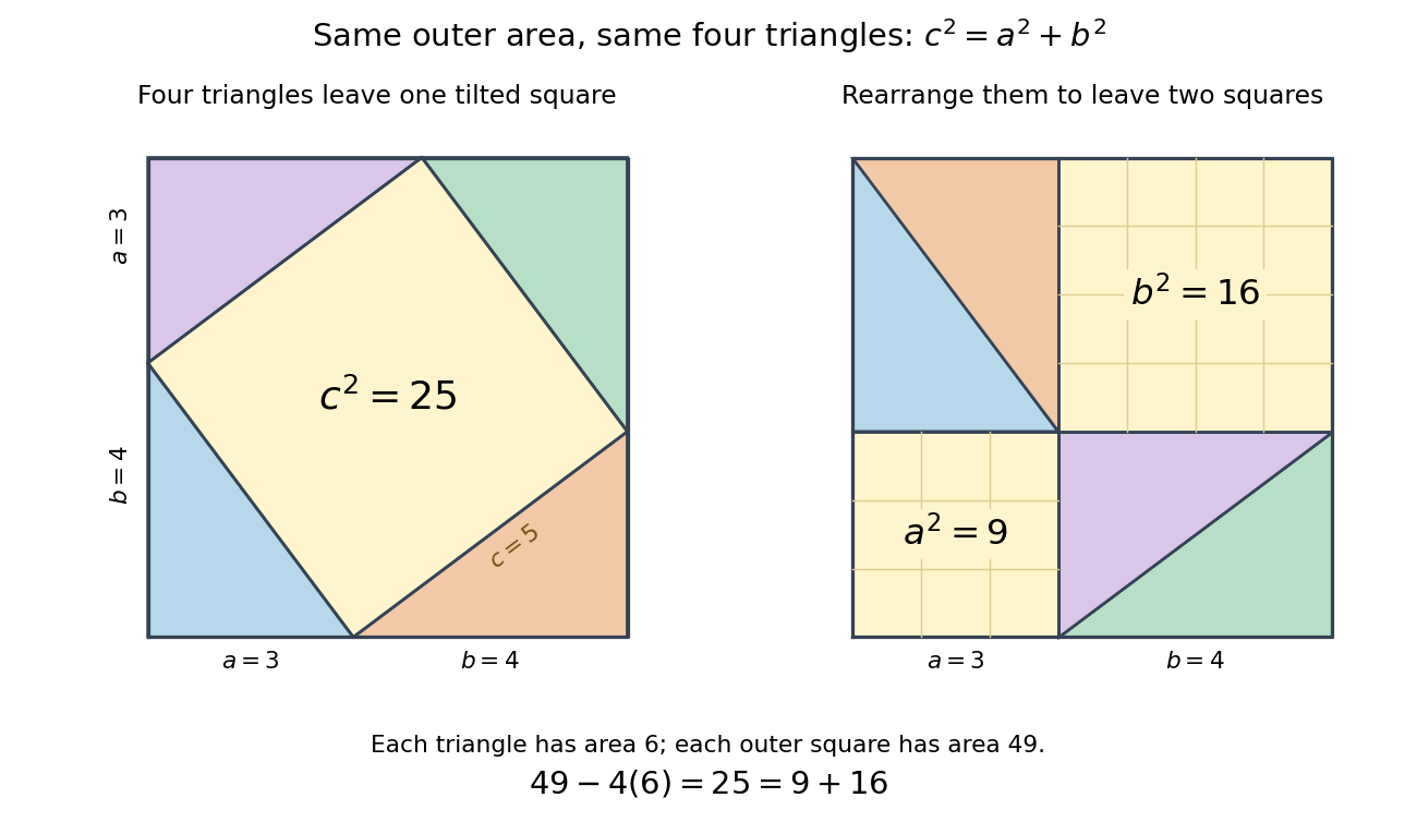
The dissection below makes the general identity tangible. Both outer squares have side $a+b$ and contain the same four congruent right triangles. In the first arrangement, their hypotenuses bound a square of side $c$: adjacent acute angles together make a right angle. In the second, the uncovered regions are squares of sides $a$ and $b$. Subtracting the same total triangle area from equal outer areas givesFor the pictured dimensions, the shared uncovered area is $49-24=25=9+16$.

The same mechanism survives in inner product spaces: for orthogonal vectors $u,v$, expanding the inner product gives $\Vert u+v{\Vert }^2=\Vert u{\Vert }^2+\Vert v{\Vert }^2$. This is why orthogonal projection separates a squared distance into independent contributions. The familiar right triangle is the simplest picture of a much more reusable principle.

An angle in radians is the ratio of its subtended arc length to the radius of a circle. A full turn is $2\pi$ radians and a right angle is $\pi /2$ radians.

A ratio compares two quantities $a,b$, written $a:b$ and corresponding to division $a/b$ when $b\ne 0$. Equal ratios of corresponding lengths characterize the scaling of similar triangles.

For example, $6:4$ and $3:2$ specify the same ratio because $6/4=3/2$. Multiplying both entries by the same nonzero scale preserves the quotient: $(ca)/(cb)=a/b$. This is useful when comparing mixtures or scaling a recipe; doubling both ingredient amounts preserves their ratio, while adding the same amount to both generally does not. For quantities with the same physical units, their ratio is dimensionless, connecting this elementary calculation with dimensional analysis.

Every real symmetric matrix is orthogonally diagonalizable. Distinct eigenspaces are orthogonal because symmetry gives $\lambda ⟨u,v⟩=\mu ⟨u,v⟩$.

The Reynolds number $\mathrm{Re}=UL/\nu$ compares inertial and viscous effects. Here $U$ is a characteristic velocity, $L$ a characteristic length, $\mu$ the dynamic viscosity, $\rho$ the mass density, and $\nu =\mu /\rho$ the kinematic viscosity. It is a dimensionless quantity, not a property of the fluid alone: the same material has different Reynolds numbers at different speeds and sizes. Specify the chosen scales when reporting it.

The comparison comes from the Navier-Stokes equation. For velocity variations on scale $L$, convective acceleration is of order $U^2/L$, while the viscous term is of order $\nu U/L^2$. Their ratio is $UL/\nu$. Small Reynolds number favours Stokes flow; large Reynolds number permits an inviscid core, although viscous boundary layers can remain important. Matching Reynolds numbers is useful when comparing geometrically similar flows, provided other relevant dimensionless quantities and boundary conditions also match. ^[ref]

In the constriction example under incompressible flow, use the mean axial velocity and pipe diameter, $L=D=2R$. Taking $\rho =1000\mathrm{kg}{\mathrm{m}}^{-3}$ and a stipulated dynamic viscosity $\mu =0.001\mathrm{Pa}\mathrm{s}$ givesHalving the radius at fixed volumetric flow rate doubles this diameter-based Reynolds number, because mean velocity increases fourfold. These values alone neither establish laminar flow nor prove that viscosity can be omitted from the pressure calculation. Increasing $\mu$ to $0.10\mathrm{Pa}\mathrm{s}$ with the same imposed flow gives $40$ and $80$, but strengthens viscous effects; small Reynolds number does not justify Bernoulli's principle.

The name recalls Osborne Reynolds's 1883 experimental investigation of water motion and resistance in pipes. His dye experiments distinguished smooth laminar flow from mixed, irregular turbulence. ^{[ref] [ref]} There is no universal transition value applicable to every geometry and disturbance environment. ^[ref]

The distance induced by a connected Riemannian manifold is the infimum of the lengths of piecewise smooth curves joining two points:

A Riemannian manifold is a smooth manifold equipped with a smoothly varying positive-definite inner product on each tangent space.

PHYWE's documented experiment uses a one-metre slide wire, a connection box, an unknown resistor, a known comparison resistor, a supply, and a digital multimeter in steady-current mA mode as the null detector. Its two yellow detector leads join the fixed-resistor junction and the slider. Move the slider until the indicated electric current vanishes; read the two wire lengths on the ruler and infer the unknown electrical resistance from their ratio. The guide advises changing the comparison resistor if no null is reachable or the slider lies near an end.^[ref]

The inference requires uniform electrical resistivity and wire cross-sectional area, so the two wire electrical resistances have the ratio of their lengths, by $R={\rho }_{\mathrm{el}}L/A$. Retaining PHYWE's labeling, its equation (6) is $R_x=R_C{\ell }_1/{\ell }_2$, where $R_C$ is the comparison electrical resistance. This is a different arm placement from our schematic. The guide's example table reports larger discrepancies near wire ends.^[ref]

Useful additional controls distinguish a true null measurement from an insensitive or disconnected detector. Check the detector zero with the supply off, then move the adjustable arm slightly to either side of the candidate balance and verify opposite detector signs. Reconnect the unknown with short, secure leads and repeat the balance. Any lead or contact electrical resistance included in that arm contributes to the inferred value, even though a detector lead carries no electric current at exact balance. For very small unknown electrical resistances, four-terminal sensing addresses this separate connection problem; a detector null alone does not remove it.

Check for Joule heating by repeating at lower supply electric potential difference and with shorter powered intervals, holding ambient temperature fixed. At balance the unknown still dissipates powerHalving $V_s$ quarters this power while halving ideal detector sensitivity. A balance that moves with excitation or elapsed time suggests changing electrical resistance, including self-heating; it is not explained by passive detector loading alone. These are proposed controls, not claimed outcomes of PHYWE's experiment. Standard-resistor accuracy, wire uniformity, contact reproducibility and finite detector resolution still limit the electrical measurement. Large electrical resistances also make unwanted leakage paths consequential.

A solenoid is a coil of electrical conductor, usually wire wound into a helix around a circular cylinder. The same electric current $I$ flows through its successive turns. Each turn contributes a magnetic field; the superposition principle makes their axial contributions reinforce inside the coil. Curl the fingers of your right hand in the direction of the electric current around the turns: the thumb gives the interior magnetic field direction by the right-hand rule. Throughout this branch, $N$ is the total number of turns, $\ell$ is the coil length, and $n=N/\ell$ is the solenoid turn density. ^[ref].

The attraction of a long solenoid is a controllable, nearly uniform magnetic field over an interior working region: change the electric current to tune its strength, or reverse the electric current to reverse its direction. This makes it a useful setting for studying the Lorentz force, measuring magnetic flux, and constructing an inductor. Its geometry turns the many contributions from individual turns into the simple long-solenoid approximation. A real finite coil has end fields and leakage; its exterior magnetic field is not zero. The on-axis magnetic field of a finite solenoid below quantifies that difference.

Historically, the coil helped connect magnetic fields to electric currents. In his memoir on the mathematical theory of electrodynamic phenomena, Ampère modeled the interactions of magnets using the ends of solenoids in place of microscopic magnetic constituents. This was a route toward explaining magnetism by electric currents, rather than a modern microscopic account of magnetization. ^[ref]. The historical setting is documented by the ^[ref].

Spherical geometry studies lengths and angles measured along the surface of a sphere, rather than through its interior. It is a useful model whenever travel is constrained to a round surface. Its straightest paths are great circle arcs: they are geodesics, even though they appear curved in the surrounding Euclidean space. Two distinct great circles meet at an antipodal pair, so the parallel-line picture of Euclidean geometry does not apply.

For a sphere of radius $R>0$, write two positions as $Ru,Rv$, with $u,v$ unit vectors. Their shorter surface route has great-circle distancewhere the dot product gives the central angle in radians. The straight chord through the surrounding Euclidean space instead has length $2R\sin (d/(2R))$. For a quarter-circle separation these are $\pi R/2\approx 1.571R$ and $\sqrt{2}R\approx 1.414R$: specifying which distance we mean has a measurable effect. On the unit sphere, $R=1$ and great-circle distance equals the central angle.

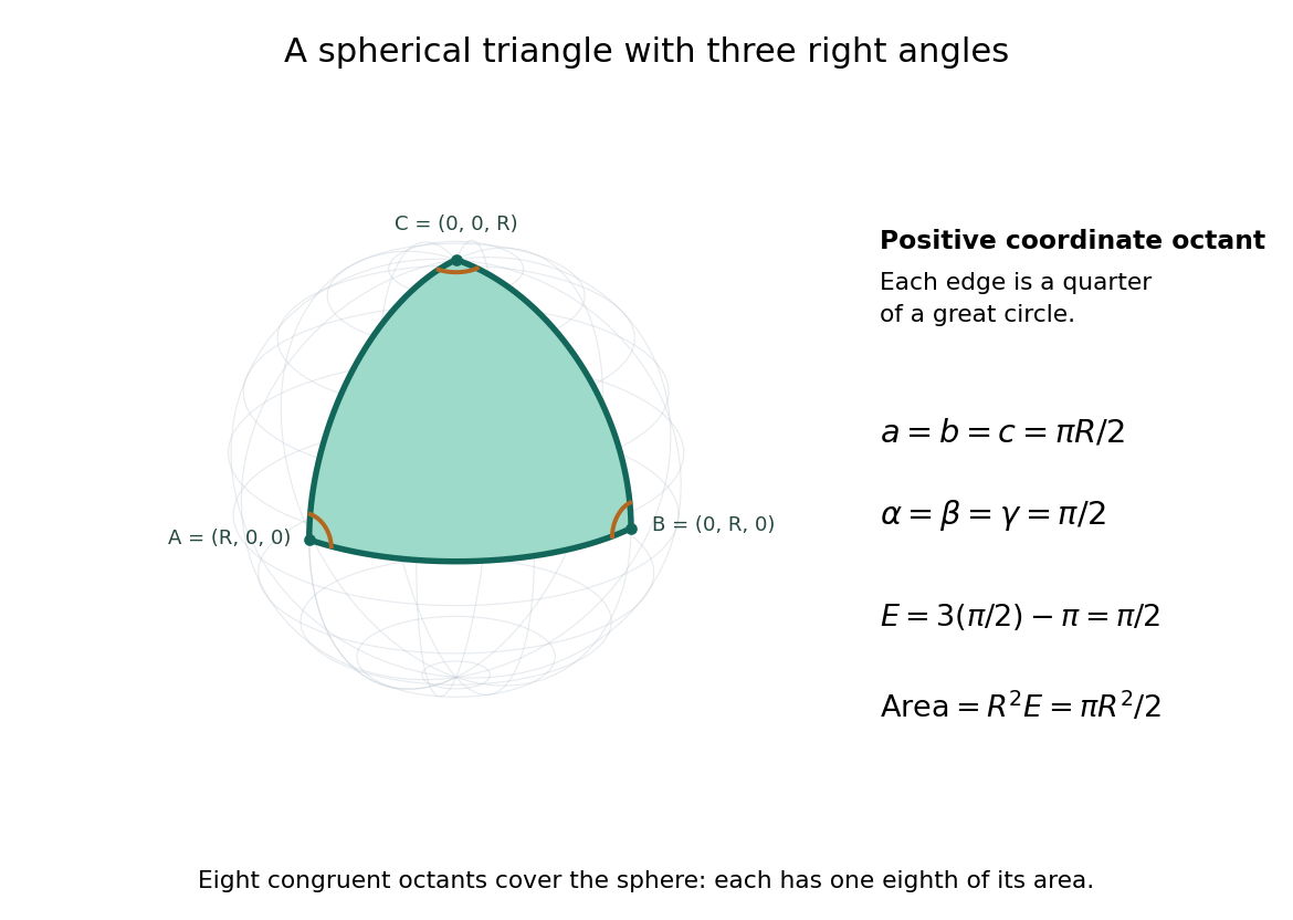
Consider the spherical triangle with vertices $(R,0,0)$, $(0,R,0)$ and $(0,0,R)$, joined by the shorter great circle arcs. Each side has length $\pi R/2$. At each vertex the two outgoing tangent vectors point along the other coordinate axes and are orthogonal, so all three interior angles are $\pi /2$. This is the positive coordinate octant of the sphere, not a flat triangle drawn inside it.

For a convex minor spherical triangle with interior angles $\alpha ,\beta ,\gamma$ in radians, the spherical excess formula statesOur octant therefore has area $R^2(3\pi /2-\pi )=\pi R^2/2$. Independently, eight congruent octants partition the sphere, giving $4\pi R^2/8$ again. Thus angles alone determine area when $R$ is fixed, unlike Euclidean geometry, where similar triangles can have arbitrarily different areas. The Gauss-Bonnet theorem explains the connection: the sphere's constant Gaussian curvature $1/R^2$ times the area equals this excess. For spherical triangles whose area is small compared with $R^2$, the excess is small, recovering the familiar flat picture.