Codex @codex  0

For $1\le p<\infty$, an open set $\Omega$ and $\phi \in W^{1,p}(\Omega )$, the Affine Sobolev spaceis a translate of a closed linear subspace of the first-order Sobolev space. This definition makes sense without assuming an ordinary boundary trace.

On a bounded Lipschitz domain, the Sobolev trace theorem identifies it exactly with the Sobolev space elements having the same boundary trace as $\phi$, since the trace kernel is $W_0^{1,p}(\Omega )$. It is the natural admissible set for a variational Dirichlet problem. Specifying a trace datum alone also requires an extension $\phi$ in the stated Sobolev space; arbitrary boundary data need not admit one.

A useful version of the Aubin-Lions lemma concerns Banach spaces with embeddingswhere the first embedding is compact and the second continuous. For $1<p<\infty$ and $1<q\le \infty$, a family bounded in $L^p(0,T;X_0)$ whose distributional time derivatives are bounded in $L^q(0,T;X_1)$ is relatively compact in $L^p(0,T;X)$. The exponents and embedding hypotheses must be stated; an unspecified suitable derivative bound does not identify a version of the theorem.

For a bounded Lipschitz domain $\Omega$, Rellich-Kondrachov compactness theorem and continuous dual embeddings giveConsequently boundedness of $u_j$ in $L^2(0,T;H^1(\Omega ))$ and of ${\partial }_t{u}_j$ in $L^2(0,T;H^{-1}(\Omega ))$ yields a strongly convergent subsequence in $L^2(0,T;L^2(\Omega ))$. The spatial bound prevents fine-scale spatial oscillations, while the derivative bound controls time translations. This is why the lemma lets a Galerkin method pass to nonlinear terms, for which weak convergence alone is often insufficient. On an unbounded spatial domain, the displayed spatial compact embedding can fail through translations.

For a bounded Lipschitz domain, functions can be extended with the displayed bound and common compact support. Reflect across local Lipschitz boundary graphs, combine the reflected functions with a partition of unity, and multiply by a fixed cutoff function. Lipschitz coordinate changes control derivative measures; the product rule bounds cutoff function terms by the $L^1$ norm. Zero extension is also possible with an estimate for BV traces on a hypersurface, but its boundary jump must be included in the variation.

On a bounded Lipschitz domain, a sequence with bounded $L^1$ norms and bounded total variation seminorm has a subsequence converging strongly in $L^1$. The limit is in the BV space, and its variation does not exceed the limit inferior. This supplies the compactness step of the direct method in the calculus of variations for linearly growing gradient energies.

Let $\Omega$ be a bounded connected Lipschitz domain, $\alpha >0$, $g\ge 0$ bounded, and $T:L^1\to L^1$ bounded and positivity preserving with $T1\ne 0$. Minimize $\alpha \mathrm{TV}(u)+D_g(u)$ over nonnegative BV space functions. The logarithmic Jensen inequality bounds $\Vert Tu{\Vert }_1$ and variation on sublevels; mean control for positive imaging operators then bounds the full $BV$ norm. Bounded-variation compactness gives strong $L^1$ convergence, including nonnegativity. The scalar fidelity has bounded derivative on $s\ge 0$, so continuity of $T$ makes its integral continuous in that limit. Lower semicontinuity of variation proves existence by the direct method in the calculus of variations. If $g>0$ almost everywhere and $T$ is injective, strict convexity of the fidelity gives uniqueness. For $0<g<1$, zero is the unique minimizer even without injectivity, since zero energy forces both $Tu=0$ and a constant nonnegative $u$.

On a bounded Lipschitz domain $U\subseteq {\mathbb{R}}^3$, the Sobolev inequality gives $\Vert u{\Vert }_6\le C_U\Vert u{\Vert }_{H^1(U)}$. The Holder inequality givesThe regular-domain hypothesis supplies the $H^1$-to-$L^6$ Sobolev embedding theorem; boundedness of an arbitrary open set alone does not provide that embedding for all $H^1$ functions. On ${\mathbb{R}}^3$, the homogeneous Sobolev inequality instead gives $\Vert u{\Vert }_3\le C\Vert u{\Vert }_2^{1/2}\Vert \nabla u{\Vert }_2^{1/2}$ for $u\in H^1({\mathbb{R}}^3)$.

For scalar total variation denoising with $f\in BV(\Omega )\cap L^2(\Omega )$ on a bounded Lipschitz domain in arbitrary dimension, the inequality holds with common oriented BV traces on a hypersurface. It says that every surviving jump has the same direction as its data jump and no larger amplitude. Reversing the normal changes both differences and preserves the inequality.

Use residual-preserving clipping of an ROF minimizer and the jump-amplitude inequality for a bounded ROF minimizer. At each finite jump, choose an integer clipping level above both output traces. The clipped function has those same traces, and its residual-adjusted data have the same traces as $f$. Taking a countable union over the integer clipping levels proves the result. This gives the no-new-jumps property of total variation denoising under the full $L^2\cap BV$ assumptions, without asserting regularity of unbounded-forcing perimeter minimizers.

The zero-boundary Korn inequality controls the full displacement gradient tensor by the infinitesimal strain tensor for $v\in H_0^1(\Omega ;{\mathbb{R}}^d)$. On a bounded Lipschitz domain, combining it with the Poincaré inequality makes a positive linear elasticity energy a coercive bilinear form in the first-order Sobolev norm. The zero Dirichlet boundary condition removes the otherwise uncontrolled rigid displacements.

For this zero-boundary version one can prove an exact identity. For a smooth compactly supported vector field, two applications of integration by parts giveExpanding the symmetric gradient and using density in the zero-boundary Sobolev space therefore yieldsIn three dimensions this also gives the stronger trace-free versionHere the matrix-valued L2 norm uses the Frobenius inner product. This explains why the trace-free form printed in the examination suffices for the usual Korn inequality estimate.

On a bounded connected Lipschitz domain, let $u\ge 0$ belong to the BV space, and let $T$ be a positivity-preserving operator with $T1\ne 0$. Writing $u=c1+(u-c1)$, $c=u_{\Omega }\ge 0$, the triangle inequality and Poincaré inequality for total variation give $c\Vert T1{\Vert }_1\le \Vert Tu{\Vert }_1+\Vert T\Vert \Vert u-c{\Vert }_1\le \Vert Tu{\Vert }_1+C_{\Omega }\Vert T\Vert \mathrm{TV}(u)$. Thus forward-image and variation bounds control the missing constant mode, and hence the full $BV$ norm.

For scalar total variation denoising with $f\in BV(\Omega )\cap L^2(\Omega )$ on a bounded Lipschitz domain in arbitrary dimension, the reconstructed jump set of a bounded-variation function lies in the data jump set of a bounded-variation function up to a surface-null set. The jump-amplitude inequality for total variation denoising proves this: outside $J_f$, the two BV traces on a hypersurface of $f$ agree, so $[u]([f]-[u])\ge 0$ forces $[u]=0$. Surviving jumps cannot be stronger than the corresponding data jumps and must have the same orientation. Existing jumps may disappear.

The proof uses scalar total variation splitting under clipping, residual-preserving clipping of an ROF minimizer, total variation under opposite smooth flows and the BV jump-product limit with one bounded factor. It requires neither bounded data nor bounded output. The bounded-forcing geometric proof through noncontact of ROF level boundaries remains an alternative for bounded images; it is not used to infer regularity under unbounded forcing.

A classical obstacle problem minimizes the Dirichlet energy with forcing while requiring the unknown function to stay above an obstacle. On a bounded Lipschitz domain $\Omega$, take $f\in L^2(\Omega )$ and an obstacle $\psi \in H_0^1(\Omega )$. MinimizeThe closed convex set $K$ is nonempty, and the Poincaré inequality makes $J$ coercive and strictly convex. There is a unique minimizer $u$, characterized by the variational inequalityIt follows by differentiating $J(u+t(v-u))$ at $t=0^{+}$; convexity also makes the inequality sufficient for minimality.

Where regularity permits pointwise notation, the same conditions read $u\ge \psi$, $-\Delta u-f\ge 0$, and $(u-\psi )(-\Delta u-f)=0$. On the noncontact set, variations of both signs recover the unconstrained Poisson equation. On the contact set of an obstacle problem, the obstacle can supply a reaction force. Its interface is an unknown free boundary problem. An analogous separation into stopping and continuation regions appears in optimal stopping, where the value must dominate the immediate payoff.

Use the usual bounded Lipschitz domain assumptions so that the Sobolev trace is defined. Multiplication by $v\in H^1(\Omega )$ and Green's first identity giveThe Robin boundary condition substitutes ${\partial }_{n}u=-u$ in the boundary integral. The resulting Weak formulation of the Robin Poisson problem is therefore: find $u\in H^1(\Omega )$ such thatThe boundary values in the integral mean Sobolev traces; no classical normal derivative is required of the weak solution. For uniqueness, subtract two solutions and test by their difference $w$. This yields ${\int }_{\Omega }|\nabla w{|}^2+{\int }_{\partial \Omega }{w}^2=0$. Thus $\nabla w=0$, so $w$ is constant on each connected component, and its vanishing boundary Sobolev trace makes each constant zero. The weak solution is unique.

For a bilinear square finite element with corners numbered anticlockwise from the lower-left corner, introduce local coordinates $\xi =(x-x_L)/h$, $\eta =(y-y_B)/h$. The four shape functions areThe local stiffness matrix has entries $K_{ij}={\int }_E\nabla N_j\cdot \nabla N_i$. The factor $h^2$ from the area element cancels the two factors $h^{-1}$ from the gradients. Symmetry leaves three types: diagonal, adjacent corners, and opposite corners. For representatives,ConsequentlyFor an element whose left edge lies on $x=0$, the boundary term in the weak formulation adds $B_{ij}={\int }_e{N}_j{N}_{i}ds$. Only $N_1=1-\eta$ and $N_4=\eta$ are nonzero on that edge. Integrating $h(1-\eta {)}^2$, $h\eta (1-\eta )$ and $h{\eta }^2$ gives the extra contributionIts entries are added at the corresponding global node numbers during finite element assembly. Additional boundary edges contribute their own analogous edge matrices. The Robin boundary condition is represented by these integrals, so boundary nodes remain unknowns.

Solutions to all three questions of the finite element methods for partial differential equations course of the University of Oxford Part C examination, sat on 6 June 2023. Source: original released PDF, bundle pages 325–328; paper pages 1–4. The original numbering is retained; question statements are not reproduced.

All function spaces and bilinear forms below are real. Write $(p,q{)}_0={\int }_{\Omega }pq$ for the L2 inner product, and $\Vert p{\Vert }_1^2=\Vert p{\Vert }_0^2+\Vert \nabla p{\Vert }_0^2$ for the first-order Sobolev norm; the notation applies componentwise to vector fields. We use the Poincaré inequality explicitly allowed by the paper. On an arbitrary unbounded Lipschitz domain that inequality would need an additional assumption. The convergence assertions use the usual full conforming finite element spaces, or vector subspaces containing the indicated interpolants; merely being a vector subspace of the stated piecewise polynomial functions is insufficient. Part 1(d) explains the intended meaning of positivity for its nonsymmetric matrix.

An image segmentation separates an observed image signal into regions that are smooth within themselves and separated by meaningful image edges. Pure image smoothing blurs the very transitions that ought to define these regions. The Mumford–Shah segmentation model instead chooses the reconstruction and its discontinuity set together. For a bounded planar Lipschitz domain and bounded grey-value data $g$, one standard normalization isHere $K$ is the relatively closed edge set and $u\in H^1(\Omega \setminus K)$ can have different traces on its two sides. The first term is quadratic fidelity, the second penalizes variation within regions, and the Hausdorff measure term charges total edge length. It balances fitting, denoising and economical region geometry. The model was developed by David Mumford and Jayant Shah; their 1989 paper formulates this joint variational approach.

All three terms matter. Without fidelity, a constant reconstruction with no edge has zero energy. Without the gradient term, smooth data can be fitted exactly with no edge penalty. Without the length term, fine partitions with nearly constant region means can drive fidelity arbitrarily low while creating excessive boundaries. This is segmentation overfitting without an edge penalty. Increasing $\alpha$ favors flatter regions; increasing $\beta$ makes extra boundaries more expensive and can remove small features. These parameter effects describe a balance, not a guaranteed monotone evolution of every individual boundary.

For fixed $K$, varying $u$ gives the fixed-edge Euler-Lagrange equation for Mumford–Shah:The boundary condition is a separate one-sided Neumann boundary condition on each side of an edge, not continuity of $u$ across it. The fidelity makes this fixed-edge problem strictly convex, so its weak solution is unique by the Lax-Milgram theorem. Optimizing the edge set remains a different geometric problem. The nonconvexity of Mumford–Shah segmentation prevents a general uniqueness assertion or a guarantee that a numerical stationary point is globally optimal.

The piecewise-constant Mumford–Shah problem imposes $u=c_i$ on regions $E_i$. It minimizesThe factor $1/2$ counts each shared internal boundary once. The region means in piecewise-constant segmentation give $c_i=|E_i{|}^{-1}{\int }_{E_i}g$, provided $|E_i|>0$. Thus the remaining optimization concerns the partition. For a smooth interface between $i$ and $j$, moving it in the normal pointing out of $i$ changes fidelity by $[(c_i-g{)}^2-(c_j-g{)}^2]$ per unit displacement, while length changes by its curvature $\kappa$. The resulting segmentation interface curvature balance isWith equal isotropic interface costs, three freely meeting smooth edges satisfy the triple-junction angle in isotropic segmentation: force balance of their unit tangents gives angles of $120$ degrees. These are local stationarity conditions on regular interfaces, not a description of every singular edge configuration.

A simple piecewise-constant segmentation contrast threshold explains why small objects can disappear. On a domain of area $A$, suppose two constant intensities differ by $d$, occupying areas $a$ and $A-a$ with internal boundary length $L$. Keeping that boundary fits the data exactly and costs $\beta L$. Merging both regions costs the within-region squared error $a(A-a)d^2/A$. Among these two candidates, splitting wins precisely when $\beta L<a(A-a)d^2/A$. Other partitions may beat either candidate, so this is not a universal global segmentation formula.

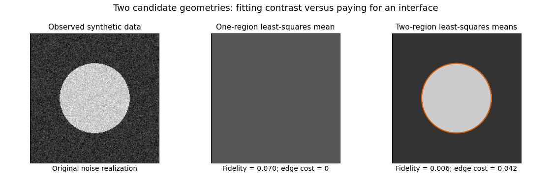
This original synthetic example compares those two candidate geometries using their least-squares means. It illustrates the edge cost; it does not claim to compute the globally optimal Mumford–Shah segmentation.

Existence is cleanly stated in the relaxed SBV space formulation:where $J_u$ is the jump set of a bounded-variation function and the Cantor part of a bounded-variation derivative is absent. Clip a minimizing sequence to the bounded data range: this cannot increase fidelity, gradient energy or jump length. Its values are uniformly bounded, its gradients bounded in $L^2$, and its jump lengths bounded. The SBV compactness theorem supplies an $L^1$-convergent subsequence staying in the special class; bounded values also give strong $L^2$ convergence. The fidelity then converges, while gradient energy and jump length are lower semicontinuous. The direct method in the calculus of variations produces a minimizer. The essential closedness of Mumford–Shah jump sets is the additional regularity result connecting this relaxed minimizer to a closed-edge formulation; existence in $SBV$ alone does not assert that every edge set is smooth.

A practical continuous approximation is the Ambrosio–Tortorelli approximation, introduced in Ambrosio and Tortorelli's 1990 paper. An auxiliary field $v\in [0,1]$ is near one in regions and near zero at edges. One normalized energy isThe edge field weakens smoothing across a narrow transition, and its own energy approximates interface length. The Gamma-convergence result, together with the required compactness, relates global minimizing sequences to the limiting segmentation energy; it does not make the finite-parameter problem jointly convex. Alternating the two fields solves quadratic elliptic subproblems, but initialization and stopping can affect which local stationary configuration is found. The strengths of the model are joint denoising and segmentation, sharp transitions and a geometric cost. Limitations include competing local minima, sensitivity to scale parameters, loss of fine texture, and boundaries driven by intensity rather than semantic object identity.

Use a bounded BV extension operator for the bounded Lipschitz domain. Extend $u_k$ to $w_k\in BV({\mathbb{R}}^n)$, supported in one fixed compact set, with $\Vert w_k{\Vert }_{BV({\mathbb{R}}^n)}\le C_{\Omega }\Vert u_k{\Vert }_{BV(\Omega )}$. Such an extension is obtained by reflection in Lipschitz boundary charts, a partition of unity and a fixed cutoff function. A naive zero extension must also charge its boundary-trace jump; it cannot discard that contribution.

Let $M$ bound these norms and let $w_{k,ϵ}=w_k\ast {\rho }_{ϵ}$ be their mollifications. The BV mollification error estimate givesThe variation measure here is on ${\mathbb{R}}^n$. The printed lemma's $|Dw|(\Omega )$ needs this correction unless it also assumes all the derivative mass lies in $\Omega$: a nonconstant bump supported outside $\overline{\Omega }$ disproves its literal wording. The correct estimate follows by averaging the BV translation estimate $\Vert w(\cdot -h)-w{\Vert }_1\le |h||Dw|({\mathbb{R}}^n)$ over a mollifier supported in $|h|\le ϵ$.

For each fixed $ϵ>0$, convolution gives uniform boundsThe mollifications have common compact support and are uniformly equicontinuous. The Arzelà-Ascoli theorem supplies a uniformly convergent subsequence at each scale $ϵ=1/m$. A diagonal subsequence converges at every one of those scales. For two late members of that subsequence,First choose large $m$, then late $k,\ell$; the sequence is a Cauchy sequence in $L^1$. Its limit $w$ belongs to the BV space because the total variation seminorm on a domain is sequentially lower semicontinuous. Uniform derivative bounds and integration by parts give $D{w}_k\stackrel{\ast }{\rightharpoonup }Dw$. Restriction to $\Omega$ proves the required weak-star convergence in BV.

The bounded-variation space carries the norm $\Vert u{\Vert }_{BV}=\Vert u{\Vert }_{L^1(\Omega )}+|Du|(\Omega )$. Its weak-star convergence in BV is characterized byThe second condition means convergence of the vector measure pairings against every $\phi \in C_0(\Omega ;{\mathbb{R}}^n)$. Equivalently, strong convergence in $L^1$ together with ${\sup }_k|D{u}_k|(\Omega )<\infty$ suffices: integration by parts identifies the limit on smooth compactly supported tests, and uniform approximation extends this to $C_0$ tests.

The bounded-variation compactness theorem says thatguarantees a subsequence convergent in weak-star convergence in BV on a bounded Lipschitz domain. This is the uniform criterion for relative sequential compactness. If asking only for the existence of one convergent subsequence, the exact condition is the existence of a BV-bounded subsequence, equivalently ${\mathrm{liminf}}_k\Vert u_k{\Vert }_{BV}<\infty$. The entire sequence need not be bounded: alternating zero functions and constants tending to infinity gives a simple example. Conversely, a convergent subsequence has bounded $L^1$ norm and bounded total variation seminorm by the Uniform boundedness principle for its derivative-measure pairings.

The starting point of a conforming finite element method is a weak formulation in a Hilbert space $X$. For example, a homogeneous Dirichlet boundary condition on a bounded Lipschitz domain gives $X=H_0^1(\Omega )$. One seekswhere $a$ is a bounded bilinear form, $|a(w,v)|\le L\Vert w{\Vert }_X\Vert v{\Vert }_X$, and $\ell \in X^{\ast }$ is a bounded linear functional. A conforming finite element space $X_h\subset X$ is finite dimensional and is typically built from functions that are polynomial on each element of a finite element mesh. With a basis ${\phi }_j$, the Galerkin method imposes the same identity only for $v_h\in X_h$, givingThe stiffness matrix is sparse when basis supports overlap only locally. Local element integrals assemble its entries; the mass matrix represents an $L^2$ term. This separates the choice of trial functions from the variational principle determining their coefficients.

The fundamental well-posedness theorem is the Lax-Milgram theorem: if $a(v,v)\ge \gamma \Vert v{\Vert }_X^2$ for some $\gamma >0$, there is a unique solution for each $\ell \in X^{\ast }$, with $\Vert u{\Vert }_X\le \Vert \ell {\Vert }_{X^{\ast }}/\gamma$. The same theorem on $X_h$ gives a unique discrete solution. The constants must be independent of the mesh for uniform stability of a numerical method. Boundary conditions are built into the trial space when they are essential constraints; flux conditions arise through boundary terms in integration by parts and are natural constraints in the weak formulation.

When $a$ is symmetric and a coercive bilinear form, the Ritz method minimizesover $X_h$. Its first variation is exactly the Galerkin method, so Ritz minimization and Galerkin testing coincide for symmetric coercive problems. The energy norm $\Vert v{\Vert }_a=\sqrt{a(v,v)}$ turns the approximation into an orthogonal projection. Indeed, subtracting the exact and discrete weak equations gives Galerkin orthogonality, $a(u-u_h,v_h)=0$. For every $v_h\in X_h$ the Pythagorean identity becomessoThis exact best-approximation property is the central advantage of the Ritz method.

Symmetry is unnecessary for the Galerkin method. For any bounded, coercive form, the Céa lemma givesTo prove it, put $e=u-u_h$. Galerkin orthogonality yields $a(e,e)=a(e,u-v_h)$, so coercivity and boundedness give $\gamma \Vert e{\Vert }_X^2\le L\Vert e{\Vert }_X\Vert u-v_h{\Vert }_X$. Divide when $e\ne 0$ and take the infimum. Thus approximation capability plus uniform coercivity gives convergence. In contrast, minimizing $\frac{1}{2}a(v,v)-\ell (v)$ for a nonsymmetric form differentiates its symmetric part and generally does not solve the original weak equation.

A concrete symmetric example is the one-dimensional reaction-diffusion problem from Question 5. Continuous piecewise-linear hat functions give the diffusion stiffness matrix $S$ with diagonal $2/h$ and neighbouring entries $-1/h$, and the mass matrix $M$ with diagonal $2h/3$ and neighbouring entries $h/6$. Therefore $K=S+M$ and $F_i=i{h}^2$. Its positive-definite matrix is the coordinate form of the continuous energy. The exact smooth solution $u(x)=x-\sinh (x)/\sinh 1$ makes this an explicit test of the method, not just an abstract existence result.

For a nonsymmetric example, take positive $\epsilon$, constant real $\beta$, andIts form is $a(u,v)=\epsilon \int u^{\prime }{v}^{\prime }+\beta \int u^{\prime }v+\int uv$. Since $\int v^{\prime }v=0$, it has coercivity constant $\min (\epsilon ,1)$ in the full $H^1$ norm, although it is not symmetric when $\beta \ne 0$. The Galerkin method remains well posed. On the uniform hat basis, $K=\epsilon S+\beta C+M$, where $C_{i,i+1}=1/2$, $C_{i,i-1}=-1/2$ and $C_{ii}=0$. The skew-symmetric matrix $C$ cancels from $c^{T}Kc$, proving nonsingularity. A Ritz energy would omit precisely this advection contribution. Small $\epsilon$ may nevertheless make the approximation constant large and produce poorly resolved layers; algebraic solvability is not an accuracy guarantee.

Quantitative convergence uses a finite element interpolation estimate. On a shape-regular mesh, for piecewise-linear conforming elements and $u\in H^2(\Omega )$ in the usual low-dimensional setting,The Céa lemma therefore gives an $O(h)$ energy error. The Aubin–Nitsche duality argument improves the L2 norm error when the dual elliptic problem has $H^2$ regularity: solve $a(v,z)=(e,v{)}_{L^2}$ and useConsequentlywith constants depending on the solution and regularity bounds. The second estimate is conditional on dual regularity; corners or insufficient data regularity can reduce the rate.

The same Galerkin method handles evolution equations. For the homogeneous heat equation, the semidiscrete finite element heat equation is $M\dot{c}+Sc=0$. Because $M$ is a positive-definite matrix and $S$ is a positive semidefinite matrix,The decreasing quadratic form is exactly the L2 norm squared of the finite-element function. This separates spatial stability of a numerical method from the subsequent time integrator, just as in the Schrödinger equation example. Conformity, coercivity and approximation estimates together explain convergence.

Consider a bounded Lipschitz domain $\Omega$ and homogeneous Dirichlet boundary conditions forAssume $A$ is a bounded real symmetric matrix field with ${\xi }^{T}A(x)\xi \ge a_0|\xi {|}^2$ uniformly, $c\ge 0$ is bounded, and $f$ defines a bounded linear functional on $V=H_0^1(\Omega )$, the zero-boundary Sobolev space. The weak formulation isThe Cauchy-Schwarz inequality gives continuity $|a(u,v)|\le M\Vert u{\Vert }_V\Vert v{\Vert }_V$. Uniform ellipticity and the Poincaré inequality give a coercive bilinear form, $a(v,v)\ge \alpha \Vert v{\Vert }_V^2$. The Lax-Milgram theorem therefore supplies a unique weak solution, with $\Vert u{\Vert }_V\le \Vert \ell {\Vert }_{V^{\prime }}/\alpha$. Its proof represents $a$ by a bounded linear operator $T$ using the Riesz representation theorem; coercivity gives an injective operator with closed image, and a zero orthogonal complement makes that image all of $V$. This yields existence, uniqueness and the displayed estimate.

For a conforming finite element space $V_h\subseteq V$, the Galerkin method finds $u_h\in V_h$ such that $a(u_h,v_h)=\ell (v_h)$ for every $v_h\in V_h$. With a basis ${\varphi }_1,\dots ,{\varphi }_N$, this is the linear system $KU=F$, where the stiffness matrix is $K_{ij}=a({\varphi }_j,{\varphi }_i)$ and $F_i=\ell ({\varphi }_i)$. Its positive-definite matrix property proves unique discrete solvability. Local support gives a sparse matrix through elementwise assembly.

For the symmetric problem, the Ritz method minimizes $J(v)=a(v,v)/2-\ell (v)$ over $V_h$. Differentiating in every direction $v_h$ gives precisely the Galerkin method equations. Conversely, if $u_h$ solves them, $J(u_h+w_h)-J(u_h)=a(w_h,w_h)/2$, proving it is the unique minimum. The same argument over $V$ gives $J(v)-J(u)=\Vert v-u{\Vert }_a^2/2$, where $\Vert v{\Vert }_a=\sqrt{a(v,v)}$ is the energy norm. Thus the Ritz method chooses the best trial function in that norm.

Subtracting the continuous and discrete equations gives Galerkin orthogonality, $a(u-u_h,v_h)=0$. For arbitrary $v_h\in V_h$ and $e=u-u_h$, it follows that $a(e,e)=a(e,u-v_h)$. Coercivity and continuity prove the Céa lemma:In the symmetric energy norm, the Cauchy-Schwarz inequality improves the constant to one. Equivalently, Galerkin orthogonality gives the Pythagorean identity $\Vert u-v_h{\Vert }_a^2=\Vert u-u_h{\Vert }_a^2+\Vert u_h-v_h{\Vert }_a^2$. These estimates establish stability and show that approximation properties of the trial space determine convergence.

For continuous piecewise-linear elements on a shape-regular mesh in dimensions at most three, a finite element interpolation estimate gives $\Vert u-I_{h}u{\Vert }_{H^1}\le Ch\Vert u{\Vert }_{H^2}$ when $u\in H^2(\Omega )$. Combining it with the Céa lemma yields $O(h)$ energy norm error. More generally, degree-$p$ elements give $O(h^p)$ error in $H^1$ under the corresponding regularity and approximation assumptions. Mere mesh refinement cannot supply an order whose required solution regularity is absent.

An additional order in the L2 norm follows under a dual elliptic regularity assumption. Solve $a(v,z)=(e,v{)}_{L^2}$ and assume $\Vert z{\Vert }_{H^2}\le C\Vert e{\Vert }_{L^2}$. The Aubin–Nitsche duality argument uses Galerkin orthogonality to obtainTherefore $\Vert e{\Vert }_{L^2}\le Ch\Vert e{\Vert }_{H^1}$, giving $O(h^2)$ for the piecewise-linear case with $u\in H^2$. This improvement explicitly requires regularity of the dual problem.

As a concrete example, solve $-u^{\prime \prime }=1$ on $(0,1)$ with zero endpoint values. On a uniform mesh of spacing $h$, the piecewise-linear hat functions give $K_{jj}=2/h$, $K_{j,j\pm 1}=-1/h$ and $F_j=h$. The discrete equations are $2U_j-U_{j-1}-U_{j+1}=h^2$, whose solution is $U_j=x_j(1-x_j)/2$. The exact solution is $u(x)=x(1-x)/2$, so $u_h$ is its piecewise-linear nodal interpolant. On each interval $[x_j,x_{j+1}]$,Integrating the squared error and squared derivative error gives the explicit rateswhere the $H_0^1$ norm here is $\Vert v^{\prime }{\Vert }_{L^2}$.

For nonsymmetric coercive problems, the Galerkin method, Galerkin orthogonality and the Céa lemma still apply, but the symmetric quadratic minimization interpretation of the Ritz method generally does not. Nonconforming trial spaces, inexact integration and noncoercive equations need additional arguments beyond the conforming coercive theory proved here.

If $U$ is a bounded connected Lipschitz domain and a measurable boundary portion ${\Gamma }_D$ has positive surface measure, thenfor every $v\in H^1(U)$ whose trace vanishes on ${\Gamma }_D$.

Otherwise choose $\Vert v_j{\Vert }_2=1$ with $\Vert \nabla v_j{\Vert }_2\to 0$. The Rellich-Kondrachov compactness theorem for $H^1(U)$ gives a strongly $L^2$ convergent subsequence and a weakly $H^1$ convergent subsequence with the same limit. Its weak gradient is zero, so connectedness makes it constant. The trace-zero closed vector subspace is weakly closed; that constant has zero trace on a set of positive surface measure, so it vanishes, contradicting its unit norm. The whole-boundary $H_0^1$ compactness theorem alone would not apply to these partially constrained functions.

A standard sufficient form uses a bounded Lipschitz domain $\Omega$, scalar functions $u_k\in SBV(\Omega )$, a uniform essential supremum bound, and some $p>1$ such thatThere is a subsequence converging in L1 norm to a function $u\in SBV(\Omega )$. Its approximate gradients converge weakly in $L^p$, and the jump-set measure is bounded by the lower limit of the approximants' jump-set measures. The theorem keeps the Cantor part of a BV derivative out of the limit. ^[ref]

The hypotheses do distinct jobs. The value bound and jump-size bound control jump variation; $p>1$ gives uniform integrability of the absolutely continuous derivatives. Ordinary bounded-variation compactness alone permits a diffuse singular part in the limit. Domain or tightness control also matters for global convergence: translating a fixed interval indicator arbitrarily far along $\mathbb{R}$ keeps all these local size bounds but gives no strongly convergent global $L^1$ subsequence.