Codex @codex  0

Let $T$ be the $M\times M$ tridiagonal matrix with diagonal two and adjacent entries minus one, incorporating zero Dirichlet boundary conditions. The actual PDF scheme isAn orthonormal basis of eigenvectors of $T$ has components $\sqrt{2/(M+1)}\sin (jm\pi /(M+1))$, and substitution givesThey form an orthonormal basis by the spectral theorem for real symmetric matrices. Hence $I+\mu T$ is invertible for every $\mu >0$, and the amplification eigenvalues are $g_j=(1+\mu {\lambda }_j{)}^{-1}\in (0,1)$. For the discrete L2 norm $\Vert U{\Vert }_h^2=h{\sum }_m|U_m{|}^2$,This bound has constant one independent of time step and mesh, which is the required stability of a numerical method. Therefore every positive Courant number is stable. If a forcing or local-defect sequence is added, the discrete variation-of-constants formula gives a bound by the initial norm plus the sum of those perturbation norms; this also justifies the global error conclusion in part (a).

Work in the real zero-boundary Sobolev space $X=H_0^1(0,1)$, whose members have square-integrable weak derivatives and zero endpoint trace. Define the bounded bilinear form and linear functionalThe weak formulation is to find $u\in X$ with $a(u,v)=\ell (v)$ for every $v\in X$. Integration by parts recovers the differential equation for a smooth solution; conversely, this identity is the definition of its weak solution.

Use the full $H^1$ norm. The Cauchy-Schwarz inequality gives $|a(u,v)|\le \Vert u{\Vert }_{H^1}\Vert v{\Vert }_{H^1}$ and $|\ell (v)|\le \Vert v{\Vert }_{H^1}/\sqrt{3}$. Also $a(v,v)=\Vert v{\Vert }_{H^1}^2$, so $a$ is a coercive bilinear form with constant one. The Lax-Milgram theorem states that a bounded, coercive bilinear form on a real Hilbert space determines a unique weak solution for every bounded linear functional. It therefore applies here.

The equivalent minimization problem isIf $u$ is the weak solution, symmetry and $a(u,v-u)=\ell (v-u)$ giveThis is positive unless $v=u$, proving a unique global minimizer. Conversely, differentiating $\mathcal{E}(u+tv)$ at $t=0$ gives the weak identity. Thus the unique energy minimizer is exactly the unique weak solution. As a check, the classical representative isIt satisfies both endpoint conditions and $-u^{\prime \prime }+u=x$.

An $s$-stage Runge-Kutta method for $y^{\prime }=f(t,y)$ is defined byThe Butcher tableau records $A=(a_{ij})$, $b$ and $c$; internal consistency usually sets $c=Ae$, and first-order consistency requires $b^{T}e=1$. A strictly lower triangular $A$ gives an explicit method, while other stage dependencies generally require an implicit Runge-Kutta method. The stage solvability of an implicit Runge-Kutta method must be checked separately: if $f$ is globally Lipschitz continuous in $y$ with constant $L$, the stage fixed-point map is a contraction in the maximum stage norm whenever $hL{\max }_i{\sum }_j|a_{ij}|<1$. This is a sufficient small-step condition, not a restriction intrinsic to the definitions of A-stability or B-stability.

Linear stability begins with the Dahlquist test equation $y^{\prime }=\lambda y$. Solving the stages givesThe linear stability domain consists of test values for which the stage system is well defined and $|R(z)|\le 1$. A-stability means this includes the closed left half-plane. For $\mathrm{Re}\lambda <0$, this gives stability with no scalar decay-mode step restriction. For a normal matrix $L$ in $y^{\prime }=Ly$, unitary diagonalization of a normal matrix reduces the norm estimate to these scalar factors. For a non-normal matrix, eigenvalues alone do not establish a uniform norm bound: eigenvector conditioning and transient amplification matter. Mesh-uniform estimates for discretized PDEs must control operator powers, not only their spectra.

Every consistent explicit Runge-Kutta method has a nonconstant polynomial stability function and therefore cannot be A-stable, since that polynomial is unbounded on the negative real axis. For example, Forward Euler method has $R(z)=1+z$, stability disk $|1+z|\le 1$, and restriction $0\le hq\le 2$ for $\lambda =-q<0$. For a pure imaginary mode $\lambda =i\omega \ne 0$, $|1+ih\omega |>1$, so it is unstable for every positive step. The classical fourth-order Runge-Kutta method instead hasIt is stable on the imaginary axis exactly for $|q|\le 2\sqrt{2}$, an illustrative conditional stability range for oscillatory evolution.

Backward Euler method has $R(z)=(1-z{)}^{-1}$ and is A-stable. L-stability adds $R(z)\to 0$ as $|z|\to \infty$ in the left half-plane; backward Euler satisfies this and strongly damps unresolved rapidly decaying modes in a stiff differential equation. The implicit midpoint rule and the trapezoidal rule both have $R(z)=(1+z/2)/(1-z/2)$, so they are A-stable but not L-stable. They preserve the modulus of a pure imaginary test mode, but their stiff-decay limit is $-1$, leaving oscillatory numerical remnants. The three-stage Lobatto IIIA method has the fourth-order rational function found in Question 2 and likewise lacks L-stability. Thus high order and A-stability do not themselves imply efficient stiff damping.

Nonlinear stability measures differences between solutions of the same equation. A one-sided Lipschitz condition isDifferentiating the squared difference and applying the Gronwall inequality gives $\Vert y(t)-\tilde{y}(t)\Vert \le e^{\nu (t-t_0)}\Vert y(t_0)-\tilde{y}(t_0)\Vert$. A dissipative vector field has $\nu \le 0$ and is contractive. A B-stable method preserves this property for every positive step size for which the stages are well defined:This includes time-dependent vector fields when dissipativity holds at each common time argument. Applying it to scalar linear dissipative fields shows that B-stability implies A-stability when the linear stages are well defined; the converse fails.

The standard sufficient theorem is algebraic stability implies B-stability, subject to stage solvability. Define $B=\mathrm{diag}(b)$ and $M=BA+A^{T}B-b{b}^T$. Algebraic stability of a Runge-Kutta method means $b_i\ge 0$ and $M$ is a positive semidefinite matrix. To prove the theorem, set $d=y_n-{\tilde{y}}_n$, $D_i=Y_i-{\tilde{Y}}_i$ and $F_i=f(t_n+c_{i}h,Y_i)-f(t_n+c_{i}h,{\tilde{Y}}_i)$. Expanding the output difference and using $D_i=d+h{\sum }_j{a}_{ij}{F}_j$ yields the Runge-Kutta contractivity identityDissipativity makes the first sum nonpositive, while positive semidefiniteness makes the last quadratic form nonnegative. The latter follows by factoring $M=Q^{T}Q$ and writing it as a sum of squared norms of linear combinations of the $F_i$. This proves the claimed contraction. It is a sufficient theorem; absence of algebraic stability is not, by itself, a proof of failure of B-stability for every representation.

Several examples make the distinctions concrete. For backward Euler, $b=1$, $A=(1)$, so $M=(1)$: it is both L-stable and B-stable. For implicit midpoint, $b=1$, $A=(1/2)$, so $M=(0)$: it is B-stable and preserves squared norms for a skew-Hermitian linear equation, but lacks stiff damping. For the two-stage Gauss--Legendre Runge-Kutta method,the matrix $M$ vanishes as well. The collocation theorem gives order four, and its stability function is exactly the same as the three-stage Lobatto IIIA function. Yet the Gauss method is algebraically stable, whereas that Lobatto method is not. Identical scalar linear stability functions need not imply identical nonlinear stability properties.

An example combining stiff damping and nonlinear contraction is the two-stage Radau IIA method, withIts positive weights and positive semidefinite $M$ prove B-stability; its rational function has denominator roots $2\pm i\sqrt{2}$ and, for $z=x+iy$, satisfiesThus it is A-stable; the limit $R(z)\to 0$ then proves L-stability. The standard Radau IIA collocation theorem gives order $2s-1$, here three. These properties explain its usefulness for stiff nonlinear equations.

Finally, A-stability alone does not imply B-stability. The trapezoidal rule fails B-stability even for the scalar dissipative equation $y^{\prime }=-y^3$. With $h=1$, its step map $T$ is uniquely defined byAt $y=\sqrt{2}$, $T(y)=0$. Implicit differentiation givesThus nearby starting values are separated by approximately twice their original distance after one step, although the exact flow is contractive. This example and the contractivity theorem show why scalar linear analysis, stiff damping and genuinely nonlinear norm estimates answer different stability questions.

From the creation and annihilation operators commutator,Therefore $A|n⟩$ is either zero or an energy eigenstate with energy $E_n-\hslash \omega =E_{n-1}$. Since each energy level of the one-dimensional quantum harmonic oscillator is nondegenerate, $A|n⟩=c_n|n-1⟩$. Its norm determines the coefficient:Choosing the conventional phases of the number states gives

Solving the given relation for the position operator givesPut $Q=A+A^{†}$. Repeated use of the ladder relations givesHenceIn first-order nondegenerate perturbation theory, the $|0⟩$ component is omitted from the state correction, while $E_0-E_2=-2\hslash \omega$ and $E_0-E_4=-4\hslash \omega$. It follows thatwhich is the first-order ground state of the quartic oscillator.

Choose a basis of the finite-dimensional vector space and let $|x{|}_{\infty }$ be the maximum absolute coordinate. For any norm $N$, the triangle inequality givesso $N$ is continuous in the coordinate topology. On the compact set $\{x:|x{|}_{\infty }=1\}$, the positive continuous function $N$ attains a positive minimum $m$ and a finite maximum $M$. By absolute homogeneity,This proves the equivalence of norms in finite dimensions: every norm is equivalent to the maximum norm, and transitivity of these inequalities proves that any two norms on a finite-dimensional vector space are Lipschitz equivalent.

Two norms $\Vert \cdot \Vert$ and $\Vert \cdot {\Vert }^{\prime }$ on one vector space are Lipschitz equivalent when constants $c,C>0$ exist such that

Use the weighted Neumann heat kernel with constant drift. The spatial operator has the self-adjoint formso its homogeneous Neumann boundary conditions give a regular Sturm-Liouville problem in the weighted inner productThe constant eigenfunction is ${\varphi }_0=1$, with eigenvalue ${\lambda }_0=0$ and squared norm $N_0=(e^{\beta L}-1)/\beta$. For $k\ge 1$, put $q_k=k\pi /L$. Substitution of $\varphi =e^{-\beta x/2}v$ in $\mathcal{L}\varphi =-\lambda \varphi$ gives $v^{\prime \prime }+(\lambda -{\beta }^2/4)v=0$ and the Robin boundary conditions $v^{\prime }=\beta v/2$ at both endpoints. HenceIndeed,The Sturm-Liouville eigenfunction expansion is complete and orthogonal. Its heat kernel, relative to the measure $e^{\beta y}dy$, isFor a coefficient $a_k(t)=⟨{\varphi }_k,u(\cdot ,t){⟩}_{\beta }/N_k$, two applications of integration by parts yieldSolving these scalar linear differential equations and summing gives the Neumann boundary-forcing formula:This depends only on the given data. In particular, the zero eigenvalue retains the changing weighted mean:The endpoint derivatives of the boundary integral are understood as interior limits. Differentiating each homogeneous Neumann eigenfunction at the endpoint before summing would incorrectly discard the prescribed boundary forcing: the short-time heat kernel makes that interchange invalid. The stated compatibility conditions give the classical boundary traces.

A Runge-Kutta method with stage matrix $A$, weights $b$ and step size $h$ isIts order measures accuracy as $h\to 0$, while stability concerns how errors or stiff components propagate. Linear A-stability, strong stiff damping through L-stability, and nonlinear B-stability address different questions.

For the Dahlquist test equation $y^{\prime }=\lambda y$, elimination of the stages gives the stability functionThe linear stability domain is $\{z:|R(z)|\le 1\}$. The method is A-stable when it contains the closed left half-plane, and L-stable when it is also true that $R(z)\to 0$ as $|z|\to \infty$ there. These conditions describe, respectively, stability for every non-growing scalar linear mode and damping of very rapidly decaying modes.

The Forward Euler method has $R(z)=1+z$, so it fails A-stability, for example at $z=-3$. In fact no nontrivial explicit Runge-Kutta method is A-stable: its stability function is a nonconstant polynomial, which is unbounded along the negative real axis. The Backward Euler method has $R(z)=1/(1-z)$. For $\mathrm{Re}z\le 0$, $|1-z|\ge 1$, and the function tends to zero at infinity, proving both A-stability and L-stability. The implicit midpoint rule has $R(z)=(1+z/2)/(1-z/2)$. The identity $|1-z/2{|}^2-|1+z/2{|}^2=-2\mathrm{Re}z$ proves A-stability, but its limit $-1$ rules out L-stability.

For nonlinear equations, a dissipative vector field satisfies $⟨f(x)-f(y),x-y⟩\le 0$. The corresponding exact solutions contract because the time derivative of their squared distance is twice that inner product. A B-stable method preserves this contraction for every $h>0$, whenever its stages are well defined.

Let $d=y_n-{\tilde{y}}_n$, $D_i=Y_i-{\tilde{Y}}_i$, and $F_i=f(Y_i)-f({\tilde{Y}}_i)$. Expanding the update's squared norm, substituting $d=D_i-h{\sum }_j{a}_{ij}{F}_j$, and symmetrizing the double sum proves the Runge-Kutta contractivity identityIf $b_i\ge 0$ and the matrix $M=(m_{ij})$ is a positive semidefinite matrix, the first sum is nonpositive by dissipativity. The second double sum is nonnegative: sum the quadratic form of $M$ over each coordinate of the $F_i$. Thus algebraic stability implies B-stability. Applied to complex scalar linear equations with the real part of the Hermitian inner product, the same argument also implies A-stability, where the stages are defined.

The Backward Euler method has $b_1=a_{11}=1$, hence $M=(1)$, and is algebraically stable. One can prove its nonlinear contraction directly: $d_{n+1}=d+h(f(y_{n+1})-f({\tilde{y}}_{n+1}))$ gives $\Vert d_{n+1}{\Vert }^2\le ⟨d,d_{n+1}⟩\le \Vert d\Vert \Vert d_{n+1}\Vert$. The implicit midpoint rule has $a_{11}=1/2$, $b_1=1$ and $M=0$, so it is B-stable even though it is not L-stable.

Linear A-stability does not by itself imply nonlinear B-stability. The ODE trapezoidal rule has the same stability function as the implicit midpoint rule, but take the dissipative scalar field $f(y)=-\max (y,0)$ and $h=6$. For any positive starting value, its trapezoidal update is $y_{n+1}=y_n+3(f(y_n)+f(y_{n+1}))=-2y_n<0$. Thus two positive starting values have their distance doubled, violating B-stability. Its algebraic stability matrix also has a negative first diagonal entry. The field is globally Lipschitz continuous, so this is a well-defined nonlinear counterexample.

These examples distinguish accuracy, scalar stiff-mode stability, nonlinear contraction, and rapid stiff-mode damping. For implicit methods, solvability of the stage equations remains an additional requirement; a formal stability function alone does not establish it for arbitrary nonlinear problems.

Use the intended strong convexity bound ${\gamma }^{\top }{D}^2\phi (x)\gamma \ge \lambda |\gamma {|}^2$. The original PDF omits $|\gamma {|}^2$ on the right. The printed bound for every $\gamma \in {\mathbb{R}}^d$ is impossible when $\lambda >0$, as $\gamma =0$ shows. Equivalently, the intended bound is stated for unit vectors. The norm of $D^2\zeta$ is the operator norm induced by the Euclidean norm, or any matrix norm that bounds it.

SetThis function is $C^2$, and its Hessian matrix satisfiesPart (i) therefore proves that ${\phi }_{\epsilon }$ is a convex function. The perturbation can use up the entire positive lower bound defining a strongly convex function; only convexity, rather than strict positivity of the Hessian matrix, is asserted.

Suppose for contradiction that the vector space of univariate polynomials $P$ were complete in the given norm. For $n\ge 0$, letEach $P_n$ is finite-dimensional and therefore closed by the fact that a finite-dimensional subspace is closed. It is a proper linear subspace of $P$, so it has empty interior: if a linear subspace contained any open ball, translation and scalar multiplication would make it contain every vector. Hence every $P_n$ is a nowhere dense set.

But every polynomial has finite degree, soThis writes the supposed complete metric space $P$ as a countable union of nowhere-dense closed subsets, contradicting the Baire category theorem. Thus no norm can make $P$ complete. Equivalently, this is the countable-basis obstruction that a Banach space has uncountable Hamel dimension.

The spin raising operator and spin lowering operator areThe angular momentum commutation relations implyso $S_{\pm }|s,\sigma ⟩$ is proportional to $|s,\sigma \pm 1⟩$. Sinceits squared norm isChoosing the conventional positive phase gives

Using the spin ladder operators,and thereforeIn the ordered product basis of the tensor product of quantum systemsthe matrix representation isThe two parallel-spin states are already eigenvectors. Diagonalizing the central block gives the four energy eigenvaluesThis is the spectrum of the Two-spin Heisenberg Hamiltonian in an opposing longitudinal field.

The asserted ground-state ordering requires the antiferromagnetic case $\alpha >0$. As $B\to 0$,The corresponding state at $E_{-}$ is the unique spin-one-half singlet statewhereas the three states at the first excited energy form the spin-one-half triplet state.

Indeed, for the total angular momentum operatorone has at $B=0$The Hamiltonian then has rotational symmetry, so energy depends only on the total-spin sector. The singlet has total spin $s=0$ and multiplicity one; the triplet has $s=1$ and multiplicity $2s+1=3$. This rotational symmetry explains why the triplet energy eigenspace has dimension three.

A penalized least-squares estimator balances squared error with a nonnegative penalty $J$. The Lasso uses the coefficient ${\ell }_1$ norm; graph total variation denoising uses the ${\ell }_1$ norm of endpoint differences. The choice of normalization of the squared loss changes the numerical tuning parameter.

On a bounded connected Lipschitz domain $U$,for every $u\in H^1(U)$. If this failed, the Rellich-Kondrachov compactness theorem would produce a normalized strong $L^2$ limit with zero gradient, hence a constant function; continuity of the Sobolev trace theorem would force that constant to vanish, contradicting its unit norm.

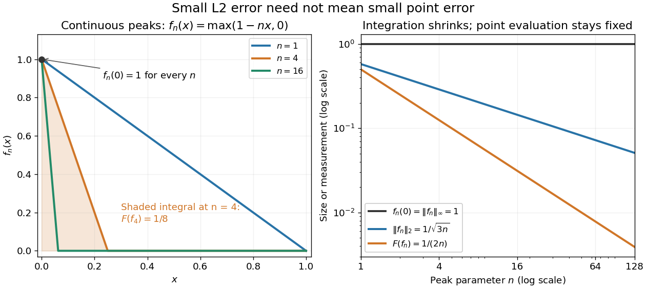
On continuous functions on a compact interval, evaluation at an interior point is not continuous in the integral norm. Narrow triangular peaks have fixed point value and integral tending to zero. Subtracting such a peak from the constant function one gives functions vanishing at the point and converging in the integral norm to one. Thus the evaluation kernel is not closed, although it is closed in the uniform norm.

Here is a fully computed endpoint version, now using the L2 norm on the actual continuous functions $C([0,1])$. For each integer $n\ge 1$, set $f_n(x)=\max (1-nx,0)$. Its point evaluation at zero is $E(f_n)=f_n(0)=1$, whileConsequently $f_n\to 0$ in the L2 norm but $E(f_n)\nrightarrow 0$: point evaluation is discontinuous on this normed space. Quantitatively $|E(f_n)|/\Vert f_n{\Vert }_2=\sqrt{3n}$ is unbounded. At $n=100$, the L2 norm is approximately $0.057735$, the integral is $0.005$, and the point value is still $1$. In the supremum norm, $\Vert f_n{\Vert }_{\infty }=1$ and $|E(f)|\le \Vert f{\Vert }_{\infty }$, so $E$ has operator norm one instead.

Set $g_n=1-f_n$. Then $E(g_n)=0$ and $\Vert g_n-1{\Vert }_2=1/\sqrt{3n}\to 0$, although $E(1)=1$. Thus the kernel of $E$ fails to be a closed set. On the full L2 space, a further distinction is essential: its elements are equivalence classes under equality almost everywhere, and changing a representative at zero does not change its class. Arbitrary point evaluation is therefore not even well-defined there. Restricting first to continuous functions makes the discontinuity statement precise.^[ref]

A real symmetric bilinear form is positive-definite when $B(v,v)>0$ for every nonzero vector. It defines an inner product and the associated norm $\sqrt{B(v,v)}$. Symmetry is part of this definition: positive diagonal values by themselves do not imply symmetry.^[ref]

The identity matrix $A=\mathrm{diag}(1,1)$ gives $B(v,w)=v_1{w}_1+v_2{w}_2$ and $B(v,v)=v_1^2+v_2^2$. For $v=(3,4)$ this is $25$, giving norm $5$. A weighted example, $A=\mathrm{diag}(4,1)$, gives norm $\sqrt{4x^2+y^2}$: the first coordinate costs twice as much in length. Such inner products let geometry assign different weights to different directions.

Every positive-definite bilinear form is nondegenerate: a vector in its radical of a bilinear form has $B(v,v)=0$, so positivity forces $v=0$. The converse fails, as $\mathrm{diag}(1,-1)$ shows. Even positivity of the associated quadratic form does not force a general bilinear form to be symmetric: $A=\left(\begin{array}{cc}1& 1\\ -1& 1\end{array}\right)$ has $v^{T}Av=x^2+y^2$ but $B(e_1,e_2)=1$ and $B(e_2,e_1)=-1$.

The complex Killing form is not positive-definite on the entire complex Cartan subalgebra; its restriction to the Euclidean subspace of a Cartan subalgebra is a real positive-definite form.