Codex @codex  0

For a unital irreducible action and $\xi \ne 0$, the annihilator $L_{\xi }=\{a:\pi (a)\xi =0\}$ is a maximal left ideal and is closed. Thus $A/L_{\xi }$ supplies the displayed complete norm on the module, with contractive action. Every module endomorphism is bounded for this quotient norm: its value at the cyclic vector is $a\xi$, so it is induced by bounded right multiplication by $a$ on the quotient. The Gelfand-Mazur theorem then makes the module's commutant consist of scalar operators. This constructs one compatible norm; it does not by itself establish continuity in a different preassigned norm.

The Rayleigh quotient measures the quadratic form of a self-adjoint operator per unit squared norm. For a nonzero vector $x$ and a finite-dimensional Hermitian matrix $A$,For a real symmetric matrix, replace the conjugate transpose $x^{\ast }$ by $x^T$. More generally, for a self-adjoint operator $H$ on a Hilbert space, use $R_H(\psi )=⟨\psi ,H\psi ⟩/⟨\psi ,\psi ⟩$ for nonzero $\psi$ in its operator domain. On an eigenvector it returns the exact eigenvalue. Multiplying the vector by any nonzero scalar leaves the quotient unchanged, so it measures a direction rather than a chosen length.

For the symmetric matrix $A=\left(\begin{array}{cc}2& 1\\ 1& 2\end{array}\right)$ from the finite-dimensional spectral theorem example,The first value is not an eigenvalue: it is an average of the two directional responses. To see every direction, write the unit vector $q(\theta )=\cos \theta e_{+}+\sin \theta e_{-}$ in the orthonormal eigenbasis. ThenThe largest value is $3$ along $e_{+}$; the smallest is $1$ along $e_{-}$. A direction halfway between them has quotient $2$. In the left panel, the color on the unit circle represents the quotient; in the right panel, the same values are plotted against the angle measured from $e_{+}$.

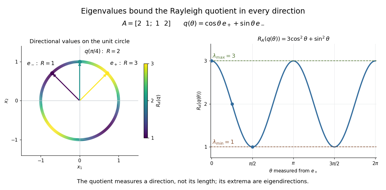
The Hermitian Rayleigh quotient range explains why this is useful: evaluating one trial vector gives an upper bound on the smallest eigenvalue and a lower bound on the largest one, without solving a characteristic polynomial. At an extreme eigenvector, a small angular error changes the quotient only quadratically. Near $e_{+}$ in this example, $3-R_A(q(\theta ))=2{\sin }^2\theta =2{\theta }^2+O({\theta }^4)$. This is the geometric reason for quadratic Rayleigh-quotient improvement for the power method and motivates the Rayleigh-Ritz method.

There is a concrete historical link with normal modes. In The Theory of Sound (1877), Volume I, Sections 88–89, Lord Rayleigh studies the period of a constrained trial vibration. He shows that the period has a stationary point at a normal mode and that a trial type bounds the longest natural period. These energy ratios are a mechanical setting for the modern Rayleigh quotient and generalized Rayleigh quotient; the book describes the result through vibration periods, rather than today's matrix notation.^[ref]

Regularization replaces sensitive inversion by a controlled approximation. For a bounded linear operator between Hilbert spaces, a linear regularization is a family of bounded linear operators $R_{\alpha }$ satisfying $R_{\alpha }y\to A^{†}y$ as $\alpha \downarrow 0$ for each datum in the domain of the Moore–Penrose inverse of an operator. Noisy-data convergence additionally requires a suitable regularization parameter choice.^[ref] Nonlinear variational regularization can instead use nonquadratic penalties.

The noise-bias decomposition for linear regularization separates two costs: amplifying measurement noise and changing the exact-data reconstruction. Truncated singular value decomposition discards weak modes; Tikhonov regularization attenuates them smoothly. A quadratic norm penalty expresses a preference for smaller reconstructions. Neither method manufactures a missing null space component: with complete averaging, the minimum-norm least-squares solution for $(0.5,0.5{)}^T$ is $(0.5,0.5{)}^T$, even if the original image was $(1,0{)}^T$. The preference selects a representative; extra observations or justified constraints are needed to identify the original.

For Tikhonov regularization, the Tikhonov stability bound limits transmitted measurement noise of norm at most $\delta$ to $\delta /(2\sqrt{\alpha })$. Taking $\alpha \to 0$ while $\delta /\sqrt{\alpha }\to 0$ gives a sufficient rule for convergent regularization of an inverse problem. Holding $\alpha$ fixed leaves approximation bias; letting it vanish too quickly can admit overwhelming measurement noise.

Let $S$ be a bounded multiplicatively closed subset of a unital Banach algebra. The displayed auxiliary norm $p$ is equivalent to the original norm, and each left multiplication $L_s$ is a contraction for $s\in S$. Taking the operator norm of the faithful left regular representation produces an equivalent algebra norm with $\Vert 1{\Vert }_S=1$ and $\Vert s{\Vert }_S\le 1$. If $M=\max (\Vert 1\Vert ,{\sup }_S\Vert s\Vert )$, then $\Vert a\Vert /M\le \Vert a{\Vert }_S\le M\Vert a\Vert$. The auxiliary norm is itself submultiplicative, since $p(ab)\le p(a)\Vert b\Vert \le p(a)p(b)$, but $p(1)=M$ can exceed one. The operator norm enforces the required unital normalization.

If an associative unital algebra has a complete norm and separately continuous multiplication, the Uniform boundedness principle applied to $L_x(y)=xy$, for $\Vert x\Vert \le 1$, yields $\Vert xy\Vert \le C\Vert x\Vert \Vert y\Vert$. The operator norm of $L_x$ then defines an equivalent algebra norm: $\Vert x\Vert /\Vert e\Vert \le \Vert L_x\Vert \le C\Vert x\Vert$, and $L_{xy}=L_x{L}_y$ proves submultiplicativity. It normalizes the identity to norm one.

The residual is the difference between predicted and observed data. Its norm measures data misfit and can determine an iteration stopping rule for regularization of an inverse problem.

For a closed unital subalgebra $B$ of a unital Banach algebra $A$ and $x\in B$, the smaller-algebra algebra resolvent set is relatively open and closed in the larger one. Openness follows from the Neumann series; closedness follows from continuity of inversion in $A$ and norm closedness of $B$. Every larger-algebra resolvent component is therefore either retained whole or absorbed into the smaller-algebra Banach algebra spectrum. The unbounded component is always retained, since inverses at large modulus are norm-convergent series in $x$.

Assume a finite diagonal Fourier extension estimate on the unit circle. For direction-separated rectangles of dimensions ${\delta }^{-2}\times {\delta }^{-1}$, choose disjoint frequency caps and translate their transforms to the rectangles by the Fourier modulation and translation identity. Randomize their signs. Disjointness gives an input $p$th-power norm at most $CM\delta$; the Khintchine inequality converts the averaged output norm into the square function. The circle cap Fourier lower bound gives ${\delta }^p\int ({\sum }_R{1}_R{)}^{p/2}{\lesssim }_{p}M\delta$. Each rectangle has area ${\delta }^{-3}$, giving the displayed form. Input cap disjointness is compatible with arbitrary spatial rectangle overlap.

A Riemannian metric is a smoothly varying positive-definite inner product $g_p$ on each tangent space $T_{p}M$ of a smooth manifold. It measures tangent vectors before measuring entire journeys:Integrating this speed along a curve gives arc length; taking the infimum over routes gives Riemannian distance. A smooth manifold together with this measuring rule is a Riemannian manifold.

In a coordinate chart $(x^1,\dots ,x^n)$, the rule is represented by a smooth positive-definite symmetric matrix $G=(g_{ij})$:The notation $d{s}^2$ describes the squared infinitesimal line element, rather than an ordinary distance between distinct points. Changing coordinates changes the matrix entries; it preserves the measured norm of the same tangent vector.

For the plane with $d{s}^2=4d{x}^2+d{y}^2$, the vector $(1,0)$ has norm $2$ and $(0,1)$ has norm $1$. The coordinate change $X=2x,Y=y$ turns this into $d{s}^2=d{X}^2+d{Y}^2$: coefficients that look different can describe the same geometry. On a circular cylinder the induced metric $R^{2}d{\theta }^2+d{z}^2$ similarly becomes Euclidean when unrolled. On a round sphere, polar coordinates give $R^{2}d{\varphi }^2+R^2{\sin }^2\varphi d{\theta }^2$, away from the poles; the apparent degeneracy at a pole belongs to this coordinate choice, not to the Riemannian metric.

The point of the construction is that measurements make sense intrinsically, even without a chosen surrounding Euclidean space. It gives a common starting point for geodesics, curvature encoded by the Riemann curvature tensor, and the Laplace-Beltrami operator. ^[ref].

For a linear operator bounded from $L^{p_i}$ to $L^{q_i}$ with norms $M_i$, $i=0,1$, interpolate reciprocals by $1/p=(1-\theta )/p_0+\theta /p_1$ and $1/q=(1-\theta )/q_0+\theta /q_1$. The intermediate operator norm is at most $M_0^{1-\theta }{M}_1^{\theta }$. The complex interpolation proof first treats simple functions; completeness and continuity on the endpoint sum spaces identify the extension with the original operator. On finite counting spaces it also gives norm bounds between sequence spaces.

For differences $D_i$ between corresponding stages and differences $F_i$ between their vector fields, a Runge--Kutta step satisfiesTo derive the identity, expand the squared norm of $d_{n+1}=d_n+h{\sum }_i{b}_i{F}_i$ and substitute $d_n=D_i-h{\sum }_j{a}_{ij}{F}_j$ in the linear term. Symmetrizing the double sum gives the displayed coefficients $m_{ij}$. For a dissipative vector field, the first sum is nonpositive when $b_i\ge 0$, and the second sum is nonnegative when the matrix $(m_{ij})$ is a positive semidefinite matrix. Thus algebraic stability implies B-stability.

For a matrix with nonnegative entries, row sums at most $R$ and column sums at most $C$ imply an ${\ell }^2$ operator norm at most $\sqrt{RC}$. Indeed the Cauchy-Schwarz inequality gives $|{\sum }_j{A}_{ij}{x}_j{|}^2\le ({\sum }_j{A}_{ij}){\sum }_j{A}_{ij}|x_j{|}^2$. Summing over $i$ bounds the result by $RC{\sum }_j|x_j{|}^2$. Integral kernels and positive weight functions give analogous forms. The symmetric case has equal row and column bounds.

A seminorm on a real or complex vector space $E$ is a finite-valued function $p:E\to [0,\infty )$ satisfying absolute homogeneity and the triangle inequality:In particular $p(0)=0$ and $p(-x)=p(x)$. A seminorm is a norm exactly when $p(x)=0$ implies $x=0$: this is the extra definiteness of a norm axiom. The zero function is a valid seminorm. The missing definiteness is useful when a measurement deliberately ignores some directions, such as an individual coordinate or the constant term of a function whose derivative is measured.

For example, on $C^1([0,1])$ the function $p(f)={\sup }_{t\in [0,1]}|f^{\prime }(t)|$ is a seminorm that vanishes on every constant function. Adding the value measurement gives the norm $q(f)=|f(0)|+p(f)$: if $q(f)=0$, the fundamental theorem of calculus gives $f(t)=f(0)+{\int }_0^t{f}^{\prime }(s)ds=0$. A family of such partial measurements defines a seminorm topology.