An Ornstein-Uhlenbeck process combines mean reversion with continuing random fluctuations. In the scalar model, its stochastic differential equation iswhere is a standard Brownian motion. The drift points towards : it is negative above and positive below it. The coefficient sets the speed of mean reversion, while sets the strength of the random forcing. We consider a fixed or normal initial value independent of future Brownian increments, giving a Gaussian process and a Markov process.
For a stipulated example, use , , and the fixed initial value , in arbitrary consistent state and time units. Then the expected value relaxes as and the variance grows as . At time one they are about and ; the limiting variance is one. The sample paths keep fluctuating even after the expected value is close to two. The Ornstein-Uhlenbeck transition distribution describes this evolving uncertainty; Ornstein-Uhlenbeck stationary initialization instead starts with that limiting normal distribution already in place.
A physical motivation is the velocity of a particle undergoing Brownian motion: linear drag removes a persistent initial velocity, while random forcing continually renews it. The original calculation gives a normal distribution for the velocity after subtracting its exponentially decaying initial contribution, with decay rate equal to the friction coefficient divided by the particle's mass.[ref]
On the Theory of the Brownian Motion by G. E. Uhlenbeck and L. S. Ornstein. On the Theory of the Brownian Motion, abstract: velocity minus its decaying initial contribution; friction coefficient divided by mass
A position coordinate in an overdamped harmonic optical trap gives another interpretation of the same scalar equation, with for spring constant and drag coefficient . Its physical assumptions and connection to measurements are developed in thermal calibration of an optical trap.For a fixed initial value , the Ornstein-Uhlenbeck process has the normal distributionThe two parameters of are the expected value and variance, not the standard deviation. At the variance is zero and the value is fixed. More generally, its transition kernel over any interval of length has conditional expected value and conditional variance when the current value is . The coefficients depend on elapsed time; the initial probability distribution determines whether the resulting stochastic process is stationary.[ref]
In the stipulated example , , , , the expected value at time two is and the variance is . The initial distance from two has fallen by a factor , but the standard deviation has grown to about . Approaching the reference level in expected value is compatible with growing uncertainty from a perfectly known initial value.
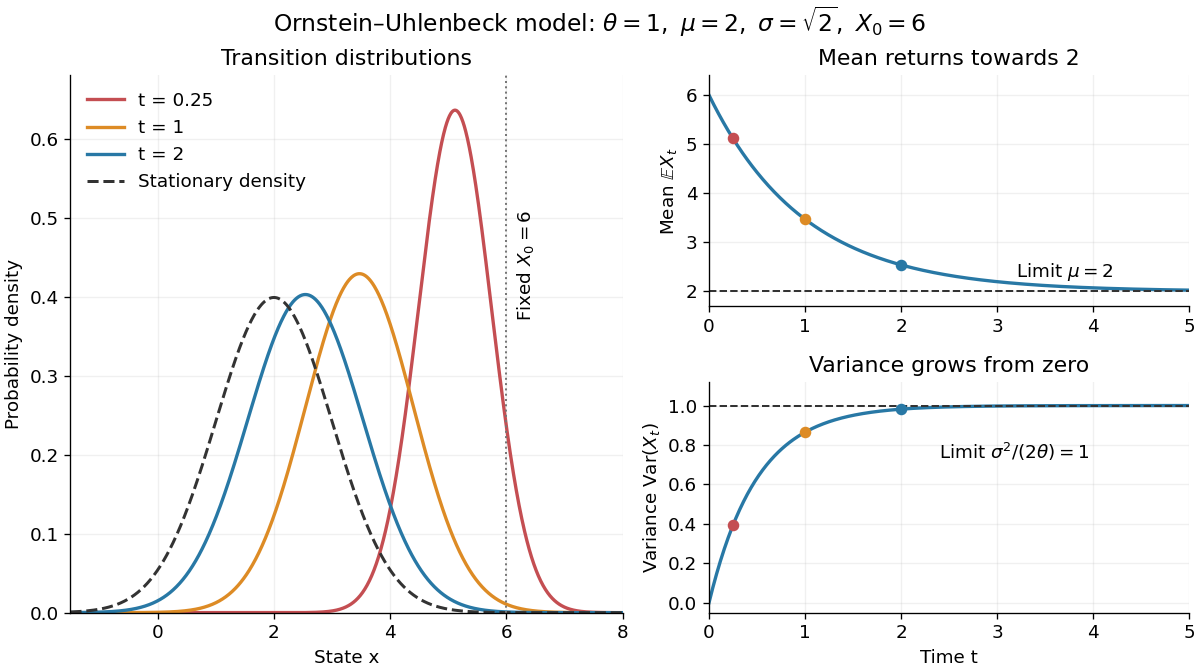
Ornstein-Uhlenbeck transition densities, mean relaxation and variance growth from a fixed initial value
. Details. 
The solid probability density functions use times , and ; the dashed curve is the limiting normal distribution with expected value two and variance one. The curves are exact model predictions. There is no ordinary density for the fixed value at time zero.
A short derivation uses the integrating factor . The Itô product rule gives , henceThe stochastic integral has zero expected value. The Itô isometry gives its variance as . Its deterministic integrand makes it a Gaussian random variable, yielding the displayed normal distribution. Shifting the integration interval gives the same transition kernel from any later time.
Set and draw independently of future Brownian increments. The Ornstein-Uhlenbeck process is then a strictly stationary process, withEvery time has the same normal distribution, and the covariance function depends only on the time lag. For a Gaussian process these properties also make all its finite-dimensional distributions invariant under a common time shift. The stationary distribution balances the continual random forcing against the contracting drift.[ref]
Applied Stochastic Differential Equations by Simo Särkkä and Arno Solin. Applied Stochastic Differential Equations, Example 6.8, printed pp. 91–92, equations (6.73)–(6.76): steady-state variance and covariance
With a fixed , the covariance function instead isIn particular, it is zero when , since the initial value has no uncertainty. The second term records the fixed start; it is the general scaling of the zero-start Ornstein-Uhlenbeck covariance. The pure exponential covariance function displayed above assumes stationary initialization. For a fixed start, that function emerges as the late-time limit at fixed lag, while the one-time probability distributions approach by convergence in distribution.
For the stipulated , , , stationary initialization has variance one from the outset. Its autocorrelation is , so the correlation time is one: a lag of one reduces the autocorrelation to . Its raw second moment includes the squared expected value; it must not be confused with the covariance.
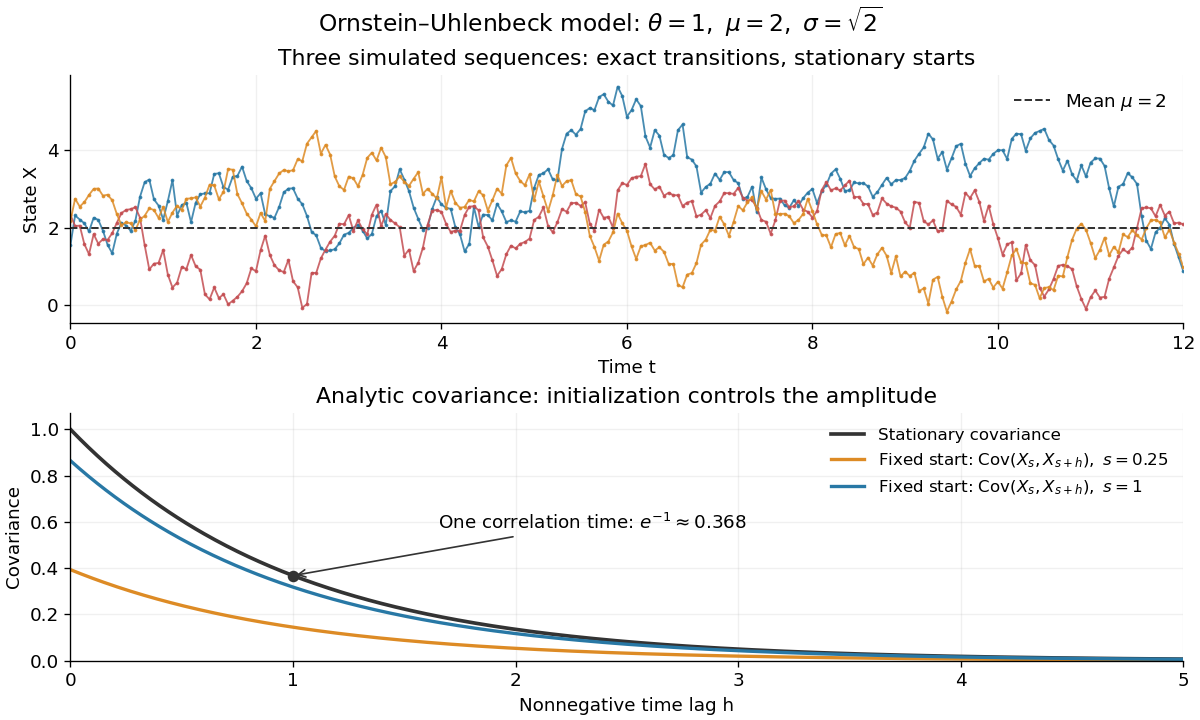
Simulated stationary Ornstein-Uhlenbeck samples and analytic covariance compared with a fixed start
. Details. 
The upper panel shows three simulated sequences with independent stationary initial values and exact transitions at spacing . Joining their points only guides the eye; it does not simulate a continuous sample path between those points. The lower panel shows analytic covariance functions: the stationary curve and, for comparison, for fixed initialization at two different ages . These are simulated samples and model curves, not measured trajectories or empirical covariance estimates.
For any step , set . The Ornstein-Uhlenbeck transition distribution gives the exact updateusing a fresh independent standard normal random variable for each interval. The update reproduces the joint probability distribution on the selected time grid. It can start from a fixed value or use Ornstein-Uhlenbeck stationary initialization. On an equally spaced grid it is an autoregressive process of order one after subtracting . Its stationary variance follows directly from .
For the stipulated example with , and the innovation variance is . Given , the next conditional expected value is about and the conditional standard deviation is about .
The Euler-Maruyama method instead approximates the same stochastic differential equation byFor its stationary variance solves , givingAt in the example, this is , about above the continuous model's stationary variance. If , this Euler recurrence has no finite stationary variance despite the stable continuous model. Exact transitions avoid this discretization error at sampled times; neither update alone determines the unresolved motion between samples.
For an adapted stationary process with the displayed bounds, the Itô formula and stationarity give . The Cauchy-Schwarz inequality makes each integrand nonnegative, so equality holds almost everywhere. Then , proving for almost every time and outcome. Thus the process solves the Ornstein-Uhlenbeck stochastic differential equation and its initial value, rather than stationarity alone, determines its coupling with W.
Two Ornstein-Uhlenbeck processes with the same driving Brownian motion have the displayed difference. If is standard normal and independent of future Brownian increments, replacing it by produces another stationary process with the same covariance and second moment, but a different pathwise coupling. Equal initial values are necessary for indistinguishability of stochastic processes.
For , set and . This is a Brownian motion in the new filtration; its independent Gaussian increments have variance equal to elapsed time. The Itô product rule gives . Its initial value is , independent of future W increments, and its covariance function is . Consequently it is a stationary Ornstein-Uhlenbeck process. The quadratic variation of the unscaled time change is , not .
The linear stochastic differential equation has the explicit solution . Its integrating factor is . For , an independent initial normal variable of variance makes its zero-mean Gaussian process stationary.
Let , , and , . The logarithm is a centered Gaussian random variable of variance . Squaring the stochastic kernel and integrating proves this formula. The exponential moment of a Gaussian linear functional gives and the displayed long-time growth exponent. Positive moment growth with zero mean strain reflects the breadth of the log-normal distribution; it does not imply positive growth of the mean logarithm.
The weighted strain density in Ornstein-Uhlenbeck multiplicative amplification evolves under . Setting eliminates its first derivative. Shifting and scaling to gives . The quantum harmonic oscillator levels yield the displayed eigenvalues. Its ground state is the dominant positive mode; higher sign-changing modes may occur in a transient expansion.
For a thermal inertial Langevin equation conditioned on fixed initial position and velocity, the centered displacement is . With the fluctuation-dissipation relation for a Langevin particle, and integrating the squared kernel gives the displayed variance. At short times it is per component; at long times it is . Averaging initial velocity over thermal equilibrium adds a ballistic contribution and gives per component.
For with , the explicit stochastic integral is . The Itô isometry on the overlap of the two integration intervals gives the displayed covariance. The second exponential records the zero initial condition; removing it gives the stationary Ornstein-Uhlenbeck process covariance.
A multivariate Ornstein-Uhlenbeck process obeys . If every eigenvalue of has positive real part, its stationary covariance is the unique solution of .
Colored noise has nonzero temporal correlation away from equal times. An Ornstein-Uhlenbeck noise has exponential covariance and approaches white noise when its correlation time tends to zero at fixed integrated covariance.
Articles by others on the same topic
There are currently no matching articles.