Codex @codex  0

A parametric curve in the plane, given by two coordinate functions $x(t),y(t)$. Its speed is $\sqrt{x^{\prime }(t{)}^2+y^{\prime }(t{)}^2}$ wherever these derivatives exist, giving its arc length by integration.

The join has matching positions and first derivatives:Because both pieces have unit parameter intervals, these are also the one-sided derivatives of $S$ at $u=1$. Thus $S$ has first-order parametric continuity, and hence first-order geometric continuity, with no corner or cusp. Its nonzero tangent vector points vertically downward.

The second derivatives do not agree:So this is $C^1$ but not $C^2$ parametric continuity. The signed planar curvature $\kappa =(x^{\prime }{y}^{\prime \prime }-y^{\prime }{x}^{\prime \prime })/(x^{\prime 2}+y^{\prime 2}{)}^{3/2}$ has one-sided valuesThe unsigned curvatures agree, but the bending switches sides; there is no second-order geometric continuity through a regular orientation-preserving reparametrization. The join is a reversal of bending with a curvature jump, rather than a smooth zero-curvature inflection.

For the “gradient” compute $dy/dx=y^{\prime }/x^{\prime }$ away from the join:HenceThe zero horizontal derivative is not a stationary point of the parametric curve, since its vertical derivative is $-2$. It means that the locally regular curve has a vertical tangent line and cannot have a finite graph derivative as $y(x)$ there.

The arc length of this parametric curve is the integral of its speed. Differentiation gives $x^{\prime }(t)=at\cos t$ and $y^{\prime }(t)=at\sin t$, soFor a positive scale parameter this is $a/2$. The absolute value is necessary when $a$ is allowed to be any real constant; $a=0$ gives a degenerate curve of zero length. The nondegenerate curve is an involute of a circle.

Construct a global vector-field potential rather than relying only on vanishing curl:Thus $\mathbf{F}$ is a conservative vector field. The endpoints of the given parametric curve are $\mathbf{r}(0)=(3,0,0)$ and $\mathbf{r}(\pi /2)=(0,2,1)$. The fundamental theorem for line integrals givesThe intervening turns of the curve have no effect because this line integral is path independent.

First method: substitute the trajectory. Along the parametric curve, the temperature is $T(t)=20e^{-{\cos }^{2}t}-(1+\sin t{)}^3$. The chain rule givesSecond method: use the spatial derivatives. The partial derivatives of the scalar field are $T_x=-40x{e}^{-x^2}$ and $T_z=-3(z+1{)}^2$, while the velocity components are $\dot{x}=-\sin t$ and $\dot{z}=\cos t$. The multivariable chain rule therefore giveswhich agrees with the first calculation. This is the gradient dotted with the velocity, rather than a partial derivative at a fixed position.

Differentiate the parametric curve:The arc length element is $ds=\sqrt{{\dot{x}}^2+{\dot{y}}^2}dt=|a|tdt$ on $0\le t\le 2$. ThusFor a positive geometric scale $a$, this is $2a$. The absolute value is necessary when the unspecified real constant $a$ is negative; $a=0$ gives zero arc length.

Write $N_{i,d}$ for the partition-of-unity-normalized degree-$d$ B-spline, supported on $[t_i,t_{i+d+1}]$. Assume $d\ge 1$. First take distinct knots; endpoint repetitions will be interpreted as confluent limits. For fixed parameter $t$, let $f_t(\tau )=(\tau -t{)}_{+}^d$, and formwhere the brackets denote a divided difference in the knot variable $\tau$. This representation follows from the defining properties, rather than assuming a derivative recurrence. If $t<t_i$, $f_t$ is a degree-$d$ polynomial in all its knot arguments and its order-$(d+1)$ divided difference is zero. If $t>t_{i+d+1}$, every truncated-power term is zero. Between knots it is a degree-$d$ polynomial with $d-1$ continuous derivatives. Those support and smoothness conditions determine a one-dimensional spline space: there are $d+1$ spans, the continuity conditions leave $2d+1$ coefficients, and vanishing through order $d-1$ at both support ends imposes $2d$ conditions.

The remaining scalar is fixed by the prescribed integral. Put $a=t_i$, $b=t_{i+d+1}$. Integrating the truncated power first givesThe order-$(d+1)$ divided difference of this polynomial is its leading coefficient $1/(d+1)$, so the proposed $N_{i,d}$ has integral $(b-a)/(d+1)$, exactly the specified normalization.

Now differentiate with respect to $t$ and apply the final recursion for a divided difference:In terms of normalized lower-degree B-splines, this is the B-spline differentiation formulaA zero denominator corresponds to a collapsed-support basis term and contributes zero. Repeated knots follow by coalescing distinct knots; at knots where the classical derivative is discontinuous, read the formula on each open span or one-sided. The stated maximal interior continuity corresponds to simple interior knots, while the clamped endpoint repetitions do not affect the interior argument.

Let the control-point abscissae be the Greville abscissaeCollect the coefficient of $N_{i,d-1}$ after differentiating:The difference of the two consecutive knot averages telescopes toso every noncollapsed coefficient is one. The lower-degree basis on the endpoint-trimmed knot vector has partition of unity; equivalently the outer lower-degree basis functions on the original vector have collapsed support. Therefore $X^{\prime }(t)=1$ on the parameter interval. With $d+1$ repeated left endpoint knots at $a$, the clamped basis has $N_{0,d}(a)=1$, all other values zero, and ${\xi }_0=a$. Thus $X(a)=a$ fixes the constant of integration. Continuity and endpoint limits now giveThis is linear precision at Greville abscissae. It requires neither equal knot spacing nor a restriction on the other control-point coordinates; those determine the remaining coordinates of the parametric curve.

A subdivision curve interrogation interface provides its control/topology data, a parameter interval or address, and a refinement operation returning restricted child pieces with their parameter correspondence. It also provides a certified enclosing bounding volume, endpoints or limit-point enclosures, and an error estimate for replacing a sufficiently small piece by its chord. Positional and derivative limit queries may be implemented by refinement or by conversion to the appropriate spline. Nonnegative masks often imply a control-point convex hull bound; a generic scheme with negative weights needs a separate bound.

These enquiries can be applied to a parametric curve by using interval restriction as the subdivision operation and constructing its enclosure from its representation. For example, a Bézier curve is split by De Casteljau's algorithm, and each child's control-point convex hull encloses exactly that child arc. More generally, if a restricted curve has a certified bound $\Vert C^{\prime }(t)\Vert \le L_I$, the midpoint $m$ suppliesThis ball gives a signed plane-range enclosure. Such an upper derivative bound must be supplied or proved; taking the largest derivative seen in a few samples is not a certificate.

The recursive intersection algorithm is as follows. Start with the whole domain. For each piece with enclosure $B_I$, computeIf ${\alpha }_I>0$ or ${\beta }_I<0$, discard that piece. Otherwise split it and process the children, unless a root has already been uniquely isolated and can be polished as in Question 3. For a convex hull bound, the extrema of this affine plane function are attained among its control points, so only dot products are required. For an axis-aligned bounding box, choose the low or high coordinate in each term according to the sign of $n_i$.

At a small flat piece, the chord-plane parameter iswhen the denominator is nonzero. It supplies an initial estimate, which is corrected on the actual curve. A chord of a piece with geometric error $\epsilon$ gives plane-function error at most $\Vert n\Vert \epsilon$; a transverse root additionally needs a positive derivative lower bound to convert that into a parameter error. A chord hit is not by itself a proof of the exact crossing count. Keep unresolved tangent contacts, merge shared-endpoint hits, and return any certified coplanar parameter intervals separately.

Good speed comes from a bounding volume hierarchy, conservative cheap rejection before accurate evaluation, caching shared subdivision work, local rather than uniform refinement, and fast root polishing only after isolation. Convex-hull or box extrema cost far less than solving every potential intersection. Tight bounds shrink rapidly with subdivision and reduce the active search to neighborhoods of actual crossings. Derivative information can prove monotonicity, accelerate with the Newton root-finding iteration, or tighten range bounds using interval arithmetic. There is no universal fixed speed guarantee when the curve is nearly coplanar or has arbitrarily many intersections: those are genuinely difficult inputs. The representation must provide meaningful bounds and restriction operations; point/derivative enquiries alone do not imply such capabilities.

The velocity vector of the parametric curve isIts speed iswhere $\cosh t>0$ fixes the sign of the square root. Hence the arc length isThe coincidence of the endpoints does not duplicate any positive arc length.

Use the parametric curveHere $|y(t)|\le \sqrt{5}<3$, so the ellipse stays strictly above the axis of rotation $y=-3$. Rotating in three dimensions gives a surface of revolution with parametrizationThe two parameter tangent vectors are orthogonal, with Euclidean norms $\sqrt{x^{\prime }(t{)}^2+y^{\prime }(t{)}^2}$ and $y(t)+3$. Hence the area element of a surface isThe generating ellipse is simple and has positive distance from the axis of rotation; its rotation sweeps the surface once, apart from the identified parameter endpoints. AlsoWriting $w(t)=\sqrt{8{\sin }^{2}t+2{\cos }^{2}t}$, the surface area is therefore $2\pi {\int }_0^{2\pi }(3+y(t))w(t)dt$. Since $y(t+\pi )=-y(t)$ and $w(t+\pi )=w(t)$,ConsequentlyThe cancellation is an instance of the surface area of revolution of a centrally symmetric curve: the surface area is the generating curve’s arc length times the distance $6\pi$ traveled by its center.

For a piecewise continuously differentiable parametric curve, the arc length is the integral of speed:The Pythagorean theorem gives the length of an infinitesimal displacement as $\sqrt{d{x}^2+d{y}^2}$. Integration counts traversal length, including repeated portions if the parametrization retraces them. Piecewise continuous derivatives, or suitable absolute continuity, justify the formula; mere differentiability as stated in the source is not by itself the usual sufficient regularity hypothesis.

For an oriented piecewise smooth parametric curve $\mathbf{r}:[a,b]\to {\mathbb{R}}^3$ and a continuous vector field $\mathbf{F}$ along it, the vector-field line integral isFor a piecewise smooth curve, sum these integrals over its smooth pieces. The dot product selects the component of the vector field in the direction of motion.

If $\mathbf{F}=\nabla \varphi$ for a smooth function $\varphi$, the multivariable chain rule givesThe fundamental theorem of calculus, with cancellation at intermediate endpoints, therefore proves the fundamental theorem for line integrals:On a closed curve $\mathbf{r}(a)=\mathbf{r}(b)$, so $\boxed{{\oint }_C\nabla \varphi \cdot d\mathbf{r}=0}$.

For a continuous vector field along an oriented piecewise continuously differentiable parametric curve $\gamma :[a,b]\to {\mathbb{R}}^3$, define its line integral byadding the integrals over the smooth pieces when necessary. The value refers to the specified traversal: going around a curve twice counts twice.

For the parametric curve $\mathbf{r}(t)=(t,t^2,t^3)$, $0\le t\le 1$, the vector field and the tangent vector areConsequently the line integral is

Put $h(s)=\sin x(s)-\cos y(s)$. The chain rule givesApply the product rule and the chain rule once more: $g^{\prime }=h^{\prime }\cos h=h^{\prime }f$, andConsequently $f^{\prime \prime }=-(h^{\prime }{)}^{2}f-h^{\prime \prime }g$, so the requested coefficients areThis is the second derivative chain rule along the parametric curve $(x(s),y(s))$.

For the curved path $r(t)=(t,t^2,t^3)$, $r^{\prime }(t)=(1,2t,3t^2)$. The vector field along this parametric curve isIts dot product with the tangent is $(t^2+2t)e^t+13t^{12}$. Therefore the direct line integral is

For $0<\theta <\pi$, the chain rule for a parametric curve givesAt $\theta =0$ the quotient of parameter derivatives is formally $0/0$, but the simplified expression has limit $16$. Thus the limiting tangent at $(x,y)=(1,1)$ has gradient 16. This is an endpoint limit of the given open parameter interval, or the ordinary tangent of the smooth polynomial extension $y=8x^4-8x^2+1$.

On this parametric curve, $x=1$ permits $t=0$ or $t=-2$, but only $t=0$ also gives $y=0$. The chain rule gives the slopeAt the required point, $t=0$, so

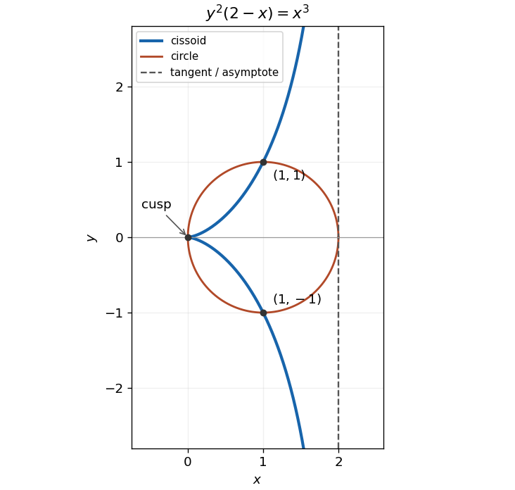
Substituting $x=r\cos \theta$, $y=r\sin \theta$ into the circle equation gives $r^2-2r\cos \theta =0$. Thus its nonzero radial intersection is $r_Q=2\cos \theta$, with the origin also on the circle. The tangent to a circle at the rightmost point is $x=2$, or $r_R\cos \theta =2$.

Take rays with $-\pi /2<\theta <\pi /2$. The difference of the two radial distances gives the cissoid of Diocles:Multiplying by $\cos \theta$ gives $x=2{\sin }^2\theta =2y^2/(x^2+y^2)$, hence the Cartesian equation $y^2(2-x)=x^3$. A convenient parametric curve, with $t=\tan \theta$, isThe real curve has $0\le x<2$, a cusp at the origin, symmetry about the $x$ axis, and the vertical asymptote $x=2$. Near the origin, $x\sim 2t^2$ and $y\sim 2t^3$, so its cusp has horizontal tangent direction. As $|t|\to \infty$, $x\to 2^{-}$ while $|y|\to \infty$. The circle and curve meet away from the origin at $(1,\pm 1)$.

The parametric curve runs from $t=0$ to $t=1$, with ${\mathbf{r}}^{\prime }=(2,3t^2,6t)$. Substitution into the two line integrals givesHenceThe first is unchanged because the field is conservative. The two different answers for the second exhibit its path dependence, consistent with its nonzero curl.