Codex @codex  0

Treat the film at fixed material content, with area $A$ the coordinate conjugate to the surface tension in the stated work term. The Helmholtz free energy is a Legendre transform of the internal energy:Its natural independent variables are therefore $T,A$, soEquality of mixed second partial derivatives gives the Maxwell relation for the thermodynamics of a liquid film:The area convention matters: the supplied fundamental relation already specifies the coefficient of $dA$. There is no additional factor of two unless one changes from total interfacial area to a projected film area and changes the work term consistently.

For a fixed amount of a simple compressible system, write the internal energy as $U(S,V)$. Its exact differential isAssuming the thermodynamic potential has continuous second partial derivatives, equality of its mixed partial derivatives yields the first Maxwell relation:For the second Maxwell relation, use the Legendre transform $H=U+pV$, the enthalpy. Its natural variables are $S,p$ sinceThus $T=(\partial H/\partial S{)}_p$ and $V=(\partial H/\partial p{)}_S$. Equality of the mixed partial derivatives now gives

The required condition is $D_{2}F(a,b)\ne 0$. The implicit function theorem then gives a unique local differentiable branch $y=f(x)$ with $f(a)=b$ andThe denominator remains nonzero after shrinking the neighborhood by continuity.

For the specified smooth function,At $(0,0)$ both equal one, so the condition holds and $f^{\prime }(0)=-1$. Differentiate $F(x,f(x))=0$ twice:At zero, $F_{xx}=F_{yy}=0$, $F_{xy}=1$, and $F_y=1$. ConsequentlyThe additional derivatives exist because this particular $F$ is smooth; the general first-derivative theorem only requires the stated continuous first partial derivatives.

The $i$th partial derivative is the limit ${\partial }_{i}f(x_0)={\lim }_{t\to 0}[f(x_0+t{e}_i)-f(x_0)]/t$. For a nonzero vector $v$, use the directional convention ${\partial }_{v}f(x_0)={\lim }_{t\to 0}[f(x_0+tv)-f(x_0)]/t$, without normalizing $v$. Differentiability means $f(x_0+h)=f(x_0)+Lh+o(\Vert h\Vert )$ for a linear map $L=df(x_0)$.

For the given example take $v=(v_1,v_2)$. If $v_1\ne 0$, then $f(tv)=t^2{v}_2^3/v_1$, so its directional difference quotient tends to zero. If $v_1=0$, the function vanishes along that line. Thus $\boxed{{\partial }_{v}f(0)=0\text{ for every }v\ne 0}$. However along $(x,y)=(t^3,t)$ with $t\ne 0$, one has $f(x,y)=1$, while $f(0,0)=0$. Hence the function is neither continuous nor differentiable at zero. Existence of all directional derivatives, even with a linear dependence on the direction, does not by itself imply total differentiability.

The $j$-th partial derivative is the vector limitwhen it exists. The total derivative is a linear map $Df(x):{\mathbb{R}}^n\to {\mathbb{R}}^m$ such thatThe Jacobian matrix is $J_f(x)=({\partial }_j{f}_i(x){)}_{i,j}$. When the total derivative exists, all partial derivatives exist and $J_f(x)$ is its matrix in the standard bases; its $j$-th column is $Df(x)e_j$. Existence of partial derivatives alone does not guarantee total differentiability.

First take the trace in four spacetime dimensions:The product rule gives $\square {\varphi }^2=2(\partial \varphi {)}^2+2\varphi \square \varphi$. For the massless equation of motion, $\varphi \square \varphi =-\lambda {\varphi }^4/6$, soBoth coefficients vanish forThe minus sign follows from the order ${\partial }^{\mu }{\partial }^{\nu }-{\eta }^{\mu \nu }\square$ used in the question's stress-energy tensor improvement. Commuting partial derivatives shows that this improvement has identically zero divergence, so it preserves the conservation law.

The precise trace identity, without using the equation of motion, isHence the massless tensor is traceless on shell. It is not traceless for arbitrary off shell configurations: a nonzero constant $\varphi =A$ with $\lambda \ne 0$ has ${\Omega }^{\mu }{}_{\mu }=\lambda A^4/6$. This is a classical result; it does not assert absence of a quantum trace anomaly.

A projective quadric is the zero locus of a nonzero homogeneous quadratic polynomial $q(v)=v^{T}Bv$, with $B$ symmetric over a field of characteristic different from two. A projective point on it is singular when all first partial derivatives vanish. Since $\nabla q(v)=2Bv$, the quadric is nonsingular exactly when $B$ is invertible.

Over the complex numbers, a nonzero quadratic form in three variables can be diagonalized by an invertible change of basis. Its rank classifies a projective conic:

The zero polynomial is excluded from the definition of a conic. Thus these last two cases are precisely the singular conics.

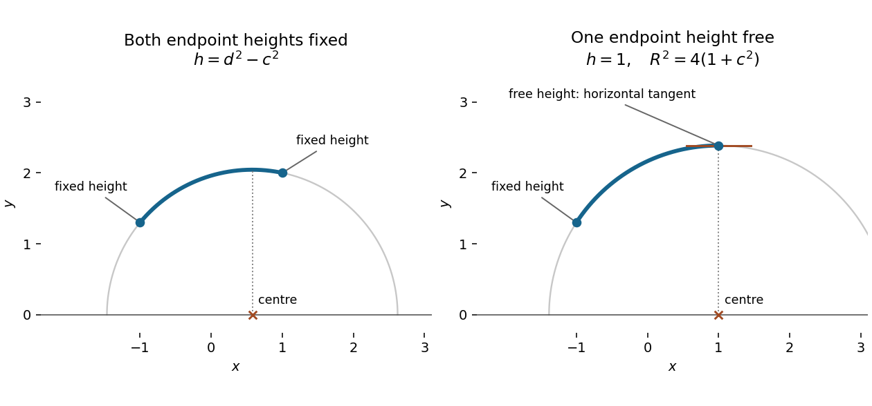
For the specified functional,Since $y>0$, the Beltrami identity gives $y\sqrt{1+y^{\prime 2}}=R$ for some $R>0$. This suggests a circular arc, but it is worth deriving its equation without dividing by $y^{\prime }$: such division would lose the point where the arc is horizontal.

Substitute the displayed partial derivative and $F_y=-\sqrt{1+y^{\prime 2}}/y^2$ in the full Euler-Lagrange equation. Combining terms over the common denominator givesThus $(y{y}^{\prime }{)}^{\prime }=-1$, so $y{y}^{\prime }=h-x$ and a second integration givesThis establishes the semicircular extremals of the hyperbolic length functional and excludes constant $y$, which would satisfy the first-order Beltrami identity for a suitable $R$ but not the full Euler-Lagrange equation.

The two prescribed endpoints giveSubtracting yields $4h=4(d^2-c^2)$. ThereforeIn particular the centre is $\boxed{(d^2-c^2,0)}$. Admissibility requires $c,d>0$, as the prescribed heights must lie in $y>0$. Under that condition the radicand is positive throughout $[-1,1]$: it is a concave quadratic polynomial whose two endpoint values are $4c^2$ and $4d^2$. The positive root consequently gives one smooth admissible arc, uniquely determined by the endpoints.

Write $a={\partial }_1{f}_1={\partial }_2{f}_2$ and $b={\partial }_2{f}_1=-{\partial }_1{f}_2$. The Cauchy-Riemann equations giveConsequentlyEquivalently, it is singular exactly when all four partial derivatives vanish. The sum of squares is over $\mathbb{R}$, so no cancellation is possible.

Let $f(X,Y)=X[r/(1+b{Y}^2)-\delta ]$. At the positive steady state, $1+b(N^{\ast }{)}^2=r/s$, where $s=\delta +1$. The two partial derivatives areThe first-order Taylor expansion with $N_t=N^{\ast }+n_t$ therefore givesEquivalently, the linearization on $(n_t,n_{t-1})$ has matrix $\left(\begin{array}{cc}1& -a\\ 1& 0\end{array}\right)$ and characteristic polynomial ${\mu }^2-\mu +a$.

Retain the material frame indifference assumption used in part (c), in addition to material isotropy. Put $p=u_{,1}$, $q=u_{,2}$ and $s=p^2+q^2$. For this antiplane shear,The invariant identities give $I_B=I{I}_B=3+s$ and $II{I}_B=1$. Hence the restriction of the strain energy density isAntiplane energy does not determine the full stress: the restriction gives one scalar energy along antiplane gradients. It does not determine the full stress derivative with respect to every entry of $F$.

Indeed, using the isotropic hyperelastic stress invariant representation and differentiating the energy, with $h_j$ denoting the corresponding partial derivatives, givesUsing $S=J^{-1}T{F}^T$, the general objective isotropic Cauchy stress tensor isAll derivatives are evaluated at the current invariant triple. The extra terms generally remain nonzero on antiplane gradients, so the printed assertion that the full stress must be $\beta B$ does not follow.

A stress-free, objective isotropic counterexample is the compressible neo-Hookean solid $W(F)=\frac{\mu }{2}(|F{|}^2-3)-\mu \log J$, with $\mu >0$. Its derivative is $T=\mu F-\mu F^{-T}$, so on antiplane gradientsTake $u(x_1,x_2)=x_1$. Then $B_{22}=1$ but $S_{22}=0$, whereas $B_{13}=1$ and $S_{13}=\mu$. The diagonal entry would force $\beta =0$, contradicting the shear entry. Thus this is not a matter of choosing the right scalar coefficient.

For the additional one-invariant constitutive assumption $W(F)=\hat{w}(I_B)$, the stronger formula does hold, withThis is a valid special case, rather than a consequence of material isotropy alone. For the general restricted energy, the shear entries are still fixed: $S_{31}=2w^{\prime }(s)u_{,1}$ and $S_{32}=2w^{\prime }(s)u_{,2}$, since $w^{\prime }=h_1+h_2$ along $(3+s,3+s,1)$. The full normal stress needs the constitutive information that the printed claim omits. If material isotropy alone is interpreted without material frame indifference, even the first reduction to $|Du{|}^2$ needs that additional material frame indifference assumption.

For a twice continuously differentiable scalar potential, mixed second partial derivatives commute. Taking the spatial curl of the equation from part (i) givesFor example, its first component is $-{\partial }_2{\partial }_3\xi +{\partial }_3{\partial }_2\xi =0$. The curl acts on the spatial representation of the material acceleration, not directly on its expression in reference coordinates.

This is a necessary local condition. It is sufficient locally, and sufficient globally on a simply connected domain under the usual smoothness assumptions. On a domain with holes, a global scalar potential additionally requires every closed-loop line integral of the material acceleration to vanish. The homogeneous motion in part (c) admits an explicit global scalar potential, so this topological qualification causes no obstruction there.

Regard $f$ as a scalar field evaluated on a specified worldline $x^{\lambda }(\tau )$. The ordinary multivariable chain rule givesThis is the directional derivative along the four-velocity. With $x^0=ct$, it reads $df/d\tau =\gamma ({\partial }_{t}f+\mathbf{v}\cdot \nabla f)$. The spatial term is present because the worldline moves through the field; it would be lost by identifying a total derivative along the particle with a partial derivative at a fixed spatial position. For a scalar the contracted expression has the same value in all coordinate systems. For a tensor field the analogous covariant derivative also transports its indices.

Write the Lorentz transformation as $x^{\prime \mu }={\Lambda }^{\mu }{}_{\nu }{x}^{\nu }$. Acting on a scalar field, the chain rule gives the four-gradientFor the specified Lorentz boost, the inverse is obtained by changing $\beta$ to $-\beta$, soThese are precisely the covector component rules for the lowered coordinates. Raising the index with the Minkowski metric ${\eta }^{\mu \nu }=\mathrm{diag}(-1,1,1,1)$ reverses the time component, yieldingIndeed ${\partial }^{\prime 0}=\gamma ({\partial }^0-\beta {\partial }^1)$ and ${\partial }^{\prime 1}=\gamma ({\partial }^1-\beta {\partial }^0)$, the contravariant four-vector rules. Thus the index on a partial derivative with respect to an upper coordinate is lower.

The four-gradient rules from a giveThe Lorentz transformation coefficients are constant, so the partial derivatives do not differentiate them. This proves the Lorentz invariance of the d'Alembert operator:For example, the two longitudinal terms transform as $-{\gamma }^2({\partial }_0+\beta {\partial }_1{)}^2+{\gamma }^2({\partial }_1+\beta {\partial }_0{)}^2=-{\partial }_0^2+{\partial }_1^2$, using ${\gamma }^2(1-{\beta }^2)=1$ and commuting partial derivatives. The transverse terms are unchanged. Applied to a scalar field, $\square$ therefore gives a Lorentz scalar.

Use $\hslash =c=1$, signature $(+---)$, and define $D_{\mu }={\partial }_{\mu }+ie{A}_{\mu }$. Under a local phase transformation,the derivative of the phase cancels the change of the potential, giving $D_{\mu }^{\prime }{\varphi }^{\prime }=e^{-ie\alpha }{D}_{\mu }\varphi$. Therefore a gauge-invariant scalar-electromagnetic Lagrangian density isThe mass term is invariant, the covariant-derivative product has canceling phases, and $F_{\mu \nu }^{\prime }=F_{\mu \nu }$ because mixed partial derivatives commute. A potential depending only on ${\varphi }^{\ast }\varphi$ may be added without changing the symmetry. The Maxwell term makes the electromagnetic field dynamical; it can be omitted when $A_{\mu }$ is a prescribed external background.

Expanding the covariant-derivative term gives the interaction linear in $e$ plus $e^2{A}_{\mu }{A}^{\mu }|\varphi {|}^2$. This quadratic term is required for exact local gauge invariance. The later part (c) deliberately gives only the linear interaction, and must be solved as that different stated Lagrangian rather than silently adding the missing term.

Assume all partial derivatives needed below are continuous. The multivariable chain rule iswhere the partial derivatives of $g$ are evaluated at $(u(x,y),v(x,y))$. Apply the product rule and the multivariable chain rule once more:Clairaut's theorem gives $g_{vu}=g_{uv}$, soDifferentiating $f_x$ with respect to $y$ instead gives

The velocity contribution in D'Alembert's formula is $\frac{1}{2}{\int }_{x-t}^{x+t}1ds=t$. Hence, with arbitrary twice continuously differentiable $h$,The added term has both second partial derivatives zero and has time derivative one, so it supplies precisely the required initial condition while preserving the wave equation.

Take each partial derivative while holding the other coordinate fixed. Differentiating the polynomial term by term givesSince the function is a polynomial, both orders of the mixed partial derivative agree everywhere.

The multivariable chain rule follows the change of both coordinates along the parametric curve:Substituting the partial derivatives from part (a), with $x=1+s^2$ and $y=e^s$, yieldsThe first term comes from changing $x$, and the remaining terms from changing $y$.