Codex @codex  0

At the origin the needed partial derivatives areThe Taylor series through total degree two is thereforewhich givesHere total degree is what matters: $x^2{y}^2$ is quartic, not quadratic. The exact omitted polynomial is $y^3+x^2{y}^2+x^2{y}^4$, which verifies the stated Big O notation remainder directly.

A critical point requires $f_x=f_y=0$. Since $y^4+y^2+1>0$ for every real $y$, the first partial derivative forces $x=0$. The second then reduces to $3y^2-3=0$, so the only critical points are $(0,1)$ and $(0,-1)$.

At these points the Hessian matrix is diagonal:The first is a positive-definite matrix, giving a strict local minimum; the second is an indefinite matrix, giving a saddle point. Their values are $f(0,1)=-1$ and $f(0,-1)=3$. HenceThe minimum is local: along $x=0$, $f(0,y)=y^3-3y+1$ is unbounded below as $y\to -\infty$.

On a branch with fixed signs of $u,v$ and $uv\ne 0$, use $u^2=x+y$ and $v^2=y-x$. Differentiating these identities, or inverting the Jacobian matrix, givesThe inverse Jacobian matrix is thereforeThese are local partial derivatives. Choosing the signs specifies an inverse function on $y>|x|$; the original map has four preimages there and has no single global inverse. At $u=0$ or $v=0$, the displayed inverse derivatives are not finite.

The requested partial derivatives areThe last printed derivative has a misplaced superscript on $f$; the second-derivative list and subsequent Taylor expansion use $f_{yy}$.

Taking the partial derivatives of the parabolic coordinates transformation, holding the other coordinate fixed each time, givesThus its Jacobian matrix is $J=\left(\begin{array}{cc}t& s\\ -s& t\end{array}\right)$.

The critical points satisfy both first partial derivatives equal to zero:Substitute $x=-y/2$ into the second equation to get $y(3y-1/2)=0$. Thus the candidates are $(0,0)$ and $(-1/12,1/6)$.

The Hessian matrix and its determinant areAt $(0,0)$ the determinant is $-1$, so the Hessian matrix is indefinite and the point is a saddle point. At $(-1/12,1/6)$ the determinant is $1$ and $h_{xx}=2>0$, so the Hessian matrix is positive definite and the point is a strict local minimum, with valueThere is no local maximum. Along $x=0$, $h(0,y)=y^3$ is unbounded above and below, so there are no global extrema either.

For a differentiable scalar function of $n$ real variables, its derivative is the linear mapwhere the column gradient is $\nabla f=(\partial f/\partial x_1,\dots ,\partial f/\partial x_n{)}^T$. Its Hessian is the $n\times n$ matrix $H_f=({\partial }^{2}f/\partial x_i\partial x_j{)}_{i,j}$. For a $C^2$ function, equality of mixed partial derivatives makes this matrix symmetric.

Put $\mathbf{h}=\mathbf{y}-\mathbf{x}$. For $0<t\le 1$, convexity gives $f(\mathbf{x}+t\mathbf{h})\le (1-t)f(\mathbf{x})+tf(\mathbf{y})$, henceBy the first-order form of Taylor's theorem, the right side tends to ${\mathbf{h}}^{\mathsf{T}}\nabla f(\mathbf{x})$ as $t\downarrow 0$. ThereforeThis is the supporting inequality for a differentiable convex function. The stated partial derivatives are enough: coordinate derivatives give directional Taylor expansion for convex functions, so no unmentioned continuity assumption on the second partial derivatives is needed. The result in fact needs less smoothness than the question assumes.

The denominator is positive throughout the domain. Holding $y$ fixed, differentiate with respect to $x$:At the interior point $(1,1/2)$ this second partial derivative is $-2/9<0$, so the restriction to a horizontal line is locally strictly concave, ruling out convexity. At the interior point $(1,2)$ it is $4/9>0$, ruling out concavity. Restrictions of a convex function or a concave function to every line segment must retain that property. Consequently $k$ is neither convex nor concave on its stated domain.

For a twice continuously differentiable deformation map, each row of its cofactor matrix has zero divergence in reference coordinates. In three dimensions write $(\mathrm{cof}Dy{)}_{iA}=\frac{1}{2}{\epsilon }_{ijk}{\epsilon }_{ABC}{y}_{j,B}{y}_{k,C}$. Applying ${\partial }_A$ gives terms in which a symmetric pair of second partial derivatives contracts with an antisymmetric Levi-Civita symbol, so each term vanishes. This identity is the cancellation that makes the Piola-Kirchhoff stress tensor transform force balance correctly between configurations.

Let a line collection have $M$ joints of a line collection and put $D=\lceil n{M}^{1/n}\rceil$. If $M>LD$, deleting each line with at most $D$ current joints of a line collection, together with those joints of a line collection, leaves a nonempty configuration in which every line has more than $D$ joints of a line collection. A nonzero polynomial of degree at most $D$ vanishes on the retained joints of a line collection by rank-nullity theorem. Choose one of minimum degree. Its restriction vanishes identically on every retained line, so its gradient is orthogonal to a spanning set of directions at every joint of a line collection and hence vanishes there. Each nonzero partial derivative would be a lower-degree polynomial with the same zeros, contradicting minimality. In characteristic zero, all derivatives vanishing forces a constant polynomial, another contradiction. Therefore $M\le LD$, giving the joints theorem. The argument's characteristic-zero assumption is essential to its derivative step.

In any finite-dimensional Euclidean space, this extension is a smooth function and all its partial derivatives at the origin vanish. Away from zero, repeated differentiation gives finite sums of coordinate polynomials divided by powers of $|x|$, multiplied by $e^{-1/|x{|}^2}$. Every such term is bounded in absolute value by $C|x{|}^{-N}{e}^{-1/|x{|}^2}$ near zero. Since Gaussian decay dominates every power, this bound tends to zero faster than any prescribed positive power of $|x|$. Induction using difference quotients then proves smoothness and zero derivatives of every order at zero.

The origin is nevertheless a strict global minimum, because $F(x)>0$ for $x\ne 0$. All its Taylor series coefficients vanish, so the function is not real analytic at zero. Adding a constant preserves the stationary minimum but changes the zeroth-order value. An expression written only for $x\ne 0$ has no stationary point at the excluded origin until an extension is specified.

A projective plane curve is reduced when its defining homogeneous polynomial is a squarefree polynomial, so no irreducible component is repeated. Its degree is the sum of the degrees of its distinct irreducible components. This convention is essential when bounding the number of singular points: the nonreduced equation $L^2=0$ has vanishing first partial derivatives at every point of its supporting line.

For a constant orthogonal matrix $R$, the Laplacian is unchanged by the coordinate transformation $\xi =Rx$. If $u$ is twice continuously differentiable, the chain rule givesbecause ${\sum }_i{R}_{ji}{R}_{ki}={\delta }_{jk}$ by orthogonality of the rows. Here ${\delta }_{jk}$ is the Kronecker delta. In two dimensions, the rotation matrix $\left(\begin{array}{cc}a& -b\\ b& a\end{array}\right)$ with $a^2+b^2=1$ makes the mixed partial derivatives cancel explicitly. The same argument works for reflections and translations, so the Laplacian depends on the Euclidean geometry rather than the orientation or origin of the coordinates.

For a classical solution of $\Delta u=f$ on a half-ball with zero data on its flat face, a tangential Caccioppoli inequality controls every second partial derivative having at least one tangential index. The equation recovers the remaining second normal derivative. The resulting Sobolev norm estimate has a dimension-only constant for the fixed radii one and two. Nonzero data are handled by homogenization of Dirichlet boundary data, adding the $W^{2,2}$ norm of the supplied boundary extension. No condition is imposed on the curved face because the smooth cutoff function vanishes there.

Let $f$ have continuous second partial derivatives near an interior critical point $x_{\ast }$ of an open subset of ${\mathbb{R}}^n$, with $\nabla f(x_{\ast })=0$. The Hessian matrix gives the following sufficient conditions:

A positive semidefinite or negative semidefinite Hessian matrix with a zero eigenvalue does not settle the classification. The higher-order test for separated extrema gives two quartic examples with exactly the same zero Hessian. These conditions apply to an interior critical point; a boundary optimum or a constrained optimization problem requires attention to the allowed directions. ^[ref]

The proof outline is the Taylor expansionFor a positive-definite matrix, the smallest eigenvalue supplies a positive bound proportional to $\Vert h{\Vert }^2$, which dominates the remainder for small enough $h$. Negate the function for the local maximum case. For opposite-sign eigenvalues, choose the two corresponding eigenvectors: the leading terms have opposite signs along their lines.

There are also necessary conditions. At an interior local minimum, the Hessian matrix is positive semidefinite; at an interior local maximum, it is negative semidefinite. Restriction to each straight line reduces this to the one-variable second derivative condition. Since the Laplacian is the trace of the Hessian, it is nonnegative at such a local minimum and nonpositive at such a local maximum. The sign of the Laplacian alone is insufficient: $x^2-2y^2$ has negative Laplacian but a saddle point of a scalar function at the origin.

Consider an original, explicitly normalized model of primary coma, rather than a prescription for a particular optical lens. Let $(u,v)$ be Cartesian coordinates in a circular optical pupil divided by its radius $a$, with $u^2+v^2\le 1$. Let $h=\alpha /{\alpha }_0$ be a signed small field angle divided by an arbitrary positive reference angle. With polar coordinates $u=\rho \cos \theta$, $v=\rho \sin \theta$, prescribe the wavefront errorHere $W_0$ is an arbitrary positive optical path difference scale, not a measured error. The cubic optical pupil dependence and linear field dependence are the classical Seidel form.^[ref]

In the paraxial approximation, light ray direction errors follow the transverse gradient of wavefront error. For a reference sphere a distance $L$ from the exit optical pupil in a uniform image medium of refractive index $n$, the corresponding image-error scale is $s=L{W}_0/(na)$. Choose image-error coordinate signs so the normalized displacement is $\nabla w$; reversing the convention reverses the plotted orientation. Image coordinates below are errors relative to the ideal image of this particular object point, rather than positions of different objects:The partial derivatives explain the asymmetry: opposite optical pupil points $(u,v)$ and $(-u,-v)$ land together, rather than on opposite sides of the ideal image. For $h>0$, every $X$ is nonnegative, while $Y$ can have either sign. The figures stipulate this single wavefront error, omit other optical aberrations and diffraction, and assign no instrument dimensions.

For a ring of fixed optical pupil radius $\rho$, the double-angle formulas for trigonometric functions giveThus each ring maps into a circle of radius $|h|{\rho }^2$ whose centre is displaced by $2h{\rho }^2$. Doubling $\rho$ quadruples both sizes; for $h=1$, the edge ring has centre $(2,0)$ and radius $1$, while the half-radius ring has centre $(1/2,0)$ and radius $1/4$. Superposing these displaced circles produces the comet-like envelope.

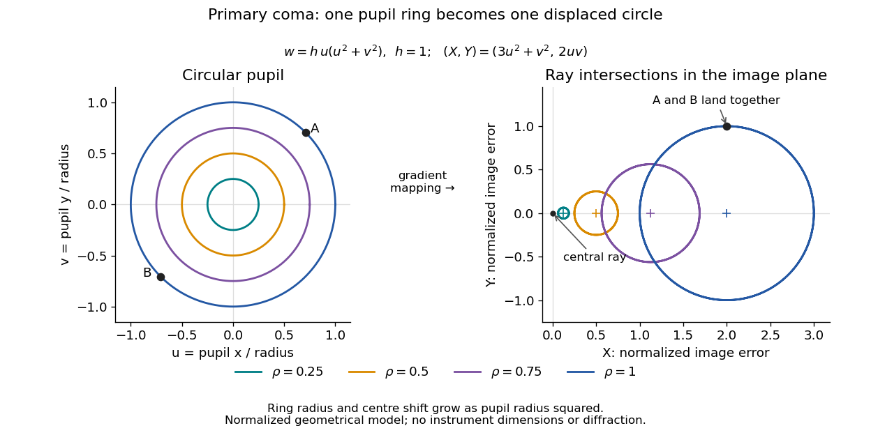
For uniform irradiance over the circular optical pupil, equal area samples give an equal-weight geometrical image. Its centroid is $(h,0)$ because $⟨u^2⟩=⟨v^2⟩=1/4$ and $⟨uv⟩=0$. Moving the coordinate origin to that centroid translates the image; it does not remove its asymmetric shape. Adding a linear term to $w$ likewise translates all light rays equally. These origin choices must be distinguished from changing the optical aberration itself.

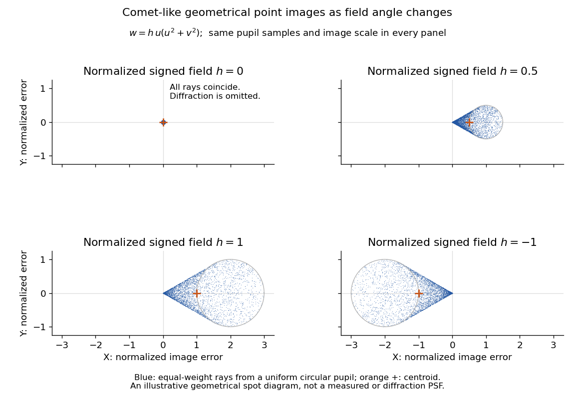
The model's full transverse extent is $3|h|$ along $X$ and $2|h|$ along $Y$. Halving the field angle halves the blur, and reversing it reverses the pattern about the ideal image. This isolates why coma matters for an optical camera's usable field of view: collecting more light does not ensure that off-axis points remain compact. Near diffraction-limited resolution, a physical optics calculation of the point spread function is needed instead of interpreting the geometrical tip as an infinitely sharp image.^[ref]

A spatial derivative is a partial derivative with respect to a spatial coordinate.

Let the atomic beam travel along $x$, with velocity $v>0$, and let $z$ measure displacement along the dominant magnetic field gradient. For a fixed effective magnetic moment component ${\mu }_z$, the magnetic dipole potential energy is $U\simeq -{\mu }_z{B}_z$. Taking its negative partial derivative givesA spatially uniform magnetic field can produce torque and Larmor precession, but cannot produce this translational separation. In a quantum state following a local internal energy eigenvalue $E_n(B)$, the more general expression is $F_z=-{\partial }_z{E}_n$, with effective magnetic moment $-\partial E_n/\partial B$. Treating that moment as constant is an approximation with a physical regime, not an extra measured fact. Assume the local magnetic field direction stays nearly fixed across the sampled beam, and that internal states follow it without transitions, as in the adiabatic theorem. The scalar gradient model describes the beam's neighborhood; it omits the full magnetic field's transverse components and fringe regions.

Assume a constant $G$ over magnet length $\ell$, followed by a field-free drift $D$. Neglect transverse motion at entry and changes in longitudinal velocity. Newton's second law gives transverse acceleration $a_z={\mu }_{z}G/M$ for whole-atom mass $M$. The magnet transit time is $t_m=\ell /v$, and the drift time is $t_d=D/v$. The magnet supplies both a displacement and an exit transverse velocity:The $\ell D$ contribution is motion with the acquired transverse velocity, not continued acceleration outside the magnet. For the plate-at-exit geometry, set $D=0$. For a nonzero entrance transverse velocity $w$, add $w(\ell +D)/v$. These terms show why initial collimation and flight geometry matter when inferring a magnetic moment from a deposit.

Choose hypothetical parameters $M=1.79\times 10^{-25}\mathrm{kg}$, $G=300\mathrm{T}{\mathrm{m}}^{-1}$, $\ell =0.035\mathrm{m}$, $D=0.100\mathrm{m}$, and $v=500\mathrm{m}{\mathrm{s}}^{-1}$. Approximate the two effective magnetic moments by ${\mu }_z=\pm {\mu }_B$, where the Bohr magneton is ${\mu }_B\simeq 9.274\times 10^{-24}\mathrm{J}{\mathrm{T}}^{-1}$. Then $|a_z|\simeq 1.55\times 10^4\mathrm{m}{\mathrm{s}}^{-2}$, $t_m=70\mu \mathrm{s}$ and $t_d=200\mu \mathrm{s}$. The positive displacement is about $0.0381\mathrm{mm}$ inside the magnet plus $0.2176\mathrm{mm}$ during drift: $d=0.2557\mathrm{mm}$, with full separation $2d=0.5114\mathrm{mm}$. These chosen values illustrate the model and are not reconstructed 1922 measurements.

The exit transverse velocity is only about $1.09\mathrm{m}{\mathrm{s}}^{-1}$, small compared with the chosen forward velocity; this checks the small-deflection assumption. Halving $G$ halves $d$, doubling $v$ divides $d$ by four, and setting $D=0$ removes most of this example's separation. A real pole has fringe magnetic fields and a position-dependent gradient; these require a more complete trajectory calculation.

If an elliptic curve has good reduction over a local field $K$, its integral projective model is smooth. Every point over the residue field lifts by the Hensel lemma, applied in a chart with a unit partial derivative. Thus reduction gives an exact sequence $0\to E_1(K)\to E(K)\to \tilde{E}(k)\to 0$. The kernel of reduction of an elliptic curve is the maximal ideal of the valuation ring, with the formal group of an elliptic curve as its group operation.