Original source: Cambridge FOI 2023/399 released PDF, physical pages 807–809.
Choose the baseline vector from the first antenna to the second. Apart from a sign convention for receiver delay, the geometric delay is , and the phase difference is . For equal received source powers , adding the voltages and averaging over many wave periods givesUncorrelated receiver noise adds a mean level but not the source's coherent cross term. For an east-west baseline and one choice of hour-angle sign, . Earth rotation therefore sweeps the phase; locally the fringe frequency is . Tracking the antenna pointing keeps the source in the primary beam. Electronic fringe stopping is a separate operation: it can remove this phase evolution, making a source at the phase centre constant in the corrected complex visibility. The oscillating power above is the geometrical fringe before that correction.
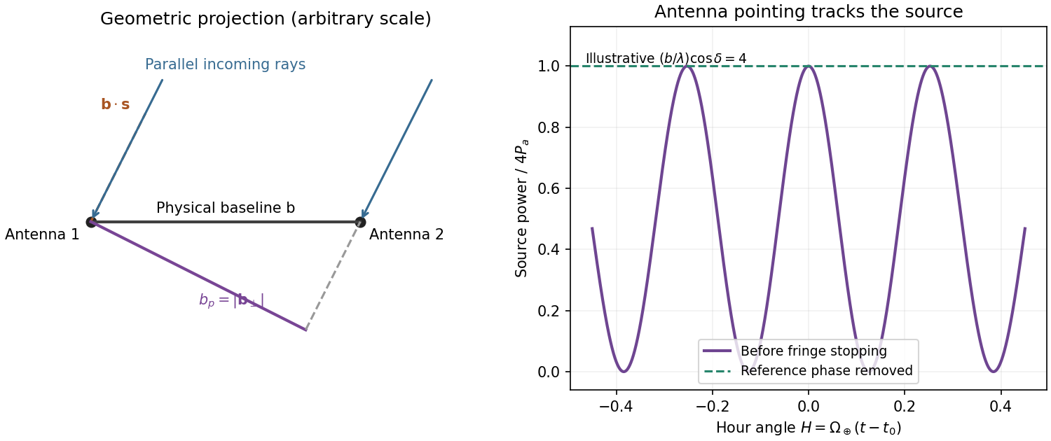
Projected interferometer baseline, geometric delay and illustrative fringes before electronic fringe stopping
. Details. 
For a small angular displacement along the projected baseline, . One full fringe therefore spans . Here . This is the angular period of the measured Fourier component and the characteristic resolution scale when such long baselines are synthesized; precise beam width and image ambiguity also depend on baseline coverage and weighting. A single pair by itself does not give an unambiguous complete image.
Writing , the expansion immediately gives the Rayleigh-Jeans law,The factor two counts the two independent modes of polarization of waves. A small brightness-temperature perturbation thus has in this limit.
Hot intracluster electrons inverse-Compton scatter the microwave-background photons. The scattering optical depth is and the characteristic thermal fractional energy transfer is of order . The integrated distortion is therefore controlled byScattering conserves photon number while shifting photons toward higher frequencies, giving a low-frequency decrement and a high-frequency increment. Thus the printed estimate correctly gives a negative change of order . Its numerical coefficient, however, is not the standard Rayleigh-Jeans coefficient. For nonrelativistic electrons and small , the Kompaneets equation gives . At small , , so andEquivalently the thermodynamic-temperature spectral factor is . The original PDF really prints the estimate with , not ; both numerical conventions are retained below. Relativistic corrections at the supplied are small compared with this factor-of-two difference.[ref]
Relativistic corrections to the Sunyaev-Zel'dovich effect by A. D. Challinor and A. N. Lasenby. abstract and Rayleigh-Jeans limit: the leading coefficient is minus twice the conventional Compton y parameter
The uniform cube has a constant line-of-sight depth . Using the supplied cross-section rather than replacing it with a more precise value givesAdopt , explicitly an external measured constant, not a temperature supplied in the question. The values , and set the physical units. Hence the printed relation gives ; the standard Rayleigh-Jeans result gives . Keeping the answer as , or twice that, avoids needing a numerical background temperature.[ref]
The Temperature of the Cosmic Microwave Background by Dale J. Fixsen. abstract, literature-combined temperature K; adopted value rounded only at the end
The face is a square, so its solid angle is , not the area of a circular six-arcminute aperture. At ,Thus using the printed estimate, or using the standard factor two. The sign denotes missing brightness relative to the surrounding microwave background. At this frequency ; the exact nonrelativistic spectral intensity differs from the strict Rayleigh-Jeans approximation by about one percent. This precision does not affect the estimates.
For the array noise, the system temperature sets the receiver noise scale; let be the effective area of each dish, and let describe correlation losses. No efficiencies or polarization of waves count are supplied, so first take and a single independent polarization of waves. An unpolarized point source produces antenna temperature , and the system-equivalent flux density is . The interferometric radiometer equation gives one baseline an rms flux error . There are cross-correlation baselines; averaging their independent thermal noise for a point source givesThe ideal single-dish effective area is , giving andCombining two independent parallel-hand polarization of waves measurements gives . Nonunit efficiencies increase these estimates by . Here signal equal to noise means a weak-source signal-to-noise ratio of one after integration; it does not mean equating the source to the entire unaveraged receiver-noise power.[ref]
Sensitivity by Joan Wrobel. 2004 Synthesis Imaging Summer School, slides 6–12 and 20: SEFD, independent baseline noise and single-polarization synthesis-image sensitivity
At the band centre, . Taking a representative maximum projected baseline of gives arcminutes. A corner-to-corner baseline of would give about arcminutes before projection and weighting. The exact antenna locations and source declination are not supplied, so neither a unique synthesized beam shape nor an exact FWHM is determined. The individual-dish primary-beam scale, roughly arcminutes, is the field of view, not the synthesized resolution.
To extract the cluster signal, retain frequency-resolved complex visibilities and fit an extended SZ template together with contaminating compact sources. For the ideal uniform square centred at the phase centre and with a nearly constant primary beam across it, the Fourier transform isThis is why the integrated decrement must not be treated as a point-source flux on every baseline. The first axial visibility null occurs at . Short baselines carry most of the large-scale decrement; the longest baselines are useful for separating unresolved positive radio sources. natural visibility weighting or a suitable taper gives a clearer extended-source image than emphasizing the longest baselines, while a visibility-domain matched filter uses all samples with weights proportional to template amplitude divided by noise variance. Its amplitude estimate is for a real template amplitude. A joint fit propagates radio-source uncertainty instead of subtracting exact, noise-free source models.
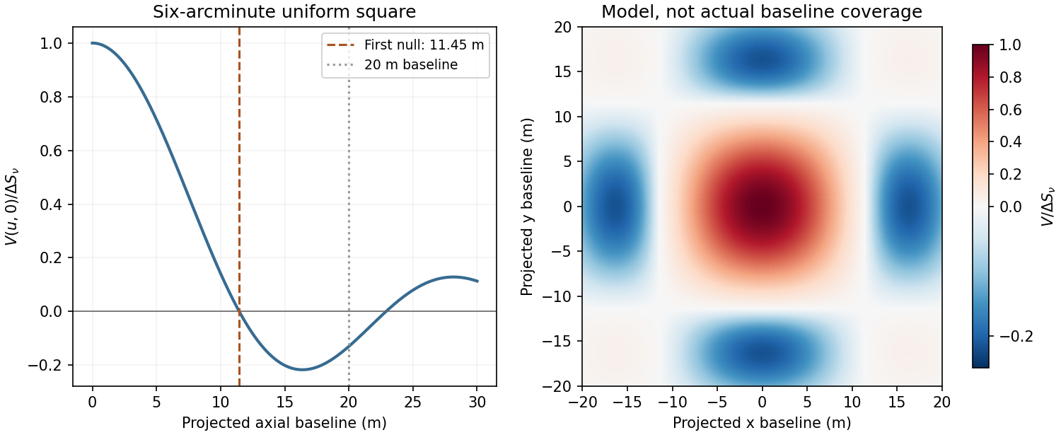
Normalized visibilities of the six-arcminute square cluster and their suppression on long baselines
. Details. 
Earth-rotation and multifrequency synthesis improve Fourier coverage, but each channel must use its own baseline in wavelengths, primary beam and SZ spectrum. Use the longer baselines and spectra to identify variable point sources, flag bad data, and test the decrement with time, antenna and frequency splits. Primary-beam and absolute-flux calibration must be included. Large-scale microwave-background fluctuations and residual ground or atmospheric signals can remain even below the thermal-noise estimate. The narrow low-frequency band alone gives limited separation of SZ and primary microwave-background temperature structure. There is no zero-spacing interferometric datum: integrated flux is model dependent unless sufficiently short baselines or additional total-power information are available. Exact cluster detection significance cannot be obtained from the point-source noise alone without the actual projected baseline distribution and weighting.
For data , parameters and model , conditional probability givesThe likelihood describes the measurement process, the prior encodes parameter information before these data, and the Bayesian evidence normalizes the posterior. A prior is a probability density with respect to a specified measure; a uniform prior in distance is not uniform in parallax. Bayes' theorem combines conditional probabilities and does not itself select an appropriate likelihood or prior.
An astronomical application starts with a forward model. For measured fluxes with predictions and known Gaussian covariance , . Correlated calibration errors belong in or in explicit calibration nuisance parameters; assuming every filter or epoch is independent can give falsely narrow uncertainties. For a faint photon-counting source, the more appropriate likelihood can instead be , with nonnegative expected source and background counts. Background measurements constrain , which is then marginalized rather than set to an exact subtracted number. The observed background-subtracted count can be negative even though the physical expected source count is nonnegative.
For a simple flux example with and a Gaussian calibration prior , completing the square givesThis explicitly shows how independent information combines. A physical nonnegative-flux prior would truncate or replace that illustrative Gaussian prior. Photometric-redshift fitting similarly compares predicted galaxy colours with measured fluxes, then integrates over luminosity, dust and other nuisance parameters to obtain . Multimodal posteriors should be retained when different spectral features produce similar colours; a best fit alone hides that ambiguity. The same framework applies to orbit parameters, stellar temperatures, cosmological parameters and cluster SZ amplitudes.
credible intervals state posterior probability conditional on the model and prior. posterior predictive checks compare replicated observations with the data and can reveal a deficient noise or source model. Sensitivity to plausible priors is especially important for weak signals and inverse problems. For competing models, posterior odds equal prior odds times the Bayes factor ; the evidence averages fit quality over the prior volume and therefore depends on proper, physically justified prior ranges. Detection thresholds and catalogue selection must enter the sampling model when inferring a population, otherwise a carefully calculated posterior can still describe a biased sample. The practical gain is a joint uncertainty distribution with nuisance parameters propagated, not merely a single fitted number.
Atmospheric refractive-index fluctuations impose a changing phase screen on the pupil. For a telescope much larger than the Fried parameter , long-exposure resolution is approximately , rather than the diffraction scale . The scaling makes the seeing width proportional to for fixed turbulence. An atmospheric coherence time sets the exposure or correction cadence needed to freeze the phase, while the isoplanatic angle sets the useful angular separation from a reference source. These are atmospheric quantities, not improvements automatically supplied by a larger mirror.
First reduce avoidable turbulence: choose a good high site, control mirror and enclosure temperatures, ventilate the dome, and observe when the line of sight crosses less turbulent air. Guiding removes telescope drift, and a fast tip-tilt correction removes image motion. Slow active optics corrects mirror figure and alignment; it cannot by itself follow all atmospheric phase fluctuations. These measures improve the input wavefront but do not guarantee diffraction-limited performance.
In adaptive optics, a wavefront sensor measures the reference-star wavefront, a reconstructor estimates its aberration, and a fast control loop commands a deformable mirror and tip-tilt element. A Shack-Hartmann sensor obtains local slopes from the displacement of focused lenslet spots. The science beam receives the corresponding optical-path correction. Residual phase variance limits the Strehl ratio approximately as when the residual is small. Enough corrected spatial modes, adequate reference photons and a response faster than atmospheric changes are all needed. infrared correction is easier because a given path error has smaller phase in radians and the atmospheric coherence length is larger. A faint or distant guide star leaves larger errors and a core-plus-halo point spread function. The NACO manual documents these reference-star and anisoplanatic limitations.[ref]
NACO User Manual by European Southern Observatory. §§3.1–3.2, printed p.13; §4.3, printed p.19: atmospheric coherence, real-time correction and anisoplanatism
A laser guide star supplies a wavefront reference in fields lacking a bright suitable star, but a finite-altitude beacon samples a cone rather than the full stellar cylinder. It also does not by itself supply the absolute celestial tip-tilt reference; a natural source is still required for that measurement. Multiple guide stars and conjugate correction planes can improve wider-field compensation, with greater hardware and reconstruction demands. The point spread function can vary across the field and with time, so reference stars and telemetry are needed to calibrate astrometry and photometry; a sharper image alone is not a guarantee of accurate science.[ref]
Adaptive Optics by European Southern Observatory. Laser guide stars: artificial reference sources, limited sky coverage and retained natural-star requirements
Short-exposure methods provide another route. Exposures shorter than the atmospheric coherence time freeze speckle patterns. speckle interferometry uses calibrated Fourier statistics of many frames to recover diffraction-scale information; phase information requires methods such as bispectrum reconstruction, not just averaging the blurred frames. lucky imaging selects the best short frames, registers them and combines them. It sacrifices photons through selection and can be read-noise limited for faint targets, so it is most effective with enough reference photons. Ordinary shift-and-add mainly corrects motion; it does not remove every high-order phase error. Deconvolution using a measured point spread function can recover supported structure but amplifies noise and cannot reliably invent spatial frequencies absent from the observations. Good-site engineering, fast wavefront correction and short-exposure reconstruction address different limitations and can be combined.
An electron accelerated in an ion's Coulomb field emits bremsstrahlung. Both electron states are unbound, giving free-free radiation rather than a discrete bound-state line. Averaging over a Maxwellian electron distribution gives an optically thin spectral emissivity with dependenceHere depends on the emissivity convention, and the Gaunt factor supplies the quantum correction. No numerical emissivity normalization is needed for these diagnostics. For a mixture, sum over ion species. The bolometric emissivity is proportional to with a frequency-averaged Gaunt factor. Thermal electron speeds control the spectrum while the encounter rate supplies its density-squared dependence.
temperature can be measured from the high-energy exponential cutoff at photon energy of order , provided the spectrum spans that turnover and foreground absorption and nonthermal contamination are modelled. At radio frequencies , the exponential is nearly one, so the optically thin continuum is a poor thermometer by slope alone. Kirchhoff's law, , and the Rayleigh-Jeans law give for an isothermal thermal plasma. The transfer solution isin the radio limit. A resolved optically thick region therefore measures its electron temperature through brightness temperature, if it fills the beam. The turnover between thick and thin emission constrains the line-of-sight emission measure for a hydrogen-dominated fully ionized plasma. In the thin regime , rather than . The slowly varying Gaunt factor gives a nearly flat optically thin radio flux-density spectrum, in contrast to the thick limit at fixed projected area.[ref]
Essential Radio Astronomy by James J. Condon and Scott M. Ransom. chapter 4, §4.3, especially equations (4.57)–(4.58): emission measure, absorption and optically thick/thin diagnostics
To obtain density, one also needs geometry. An angular extent and independent distance give a transverse size; an assumed shape provides a depth or volume. For approximately uniform emitting gas with astrophysical volume filling factor , , so . Alternatively a measured column emission measure and assumed path length give an rms density. Clumping raises the mean squared density relative to the square of the mean: the inferred value is not automatically the mean gas density. Free-free brightness alone does not uniquely determine temperature, density and physical size. Resolved imaging, a distance, optical-depth information or an independent column-density diagnostic is needed to remove those degeneracies. Cluster SZ data are complementary because their leading signal depends on , whereas free-free emission depends on density squared. Metal lines, unresolved temperature structure, foreground absorption, synchrotron emission and background subtraction must be controlled before attributing the continuum to a single thermal component.
Type Ia supernovae are standardizable candles. Repeated multiband photometry measures peak apparent magnitude, light-curve width and colour; spectra identify the supernova class and determine redshift, often from the host galaxy. Nearby objects calibrate the relation between light-curve shape, colour and absolute luminosity. Applying those relations produces a corrected apparent magnitude , not an assumption that every event has identical luminosity. The distance modulus then givesA common uncertainty in is degenerate with the absolute distance scale, but does not erase the redshift-dependent shape of the Hubble diagram.
luminosity distance probes the expansion history. In a spatially flat model,For fixed low-redshift calibration, a negative increases the second-order distance relative to a decelerating model. Objects at a given redshift are therefore fainter. A Hubble diagram spanning enough redshift can distinguish this curvature from the common magnitude intercept. In matter-plus-cosmological-constant models, ; fitting the distances can test whether . The two original supernova teams found distances supporting an accelerating expansion in that framework.[ref]
Observational Evidence from Supernovae for an Accelerating Universe and a Cosmological Constant by Adam Riess and others. abstract and cosmological interpretation of standardized supernova luminosity distances
[ref]Measurements of Omega and Lambda from 42 High-Redshift Supernovae by Saul Perlmutter and others. abstract; cosmological likelihood constraints and tests of systematic uncertainty
The comparison requires matched rest-frame passbands and K corrections, correction for redshift time dilation in the light curves, a common photometric calibration, and explicit uncertainty propagation. Dust extinction can imitate dimming; multicolour and infrared observations test reddening and the adopted extinction law. Evolution in the progenitor population or host-galaxy dependence can alter standardization, so one compares matched populations and fits host-dependent terms where warranted. Flux-limited discovery introduces Malmquist bias and other selection effects, which must be modelled through the survey detection efficiency. peculiar velocities matter at low redshift, while gravitational lensing and intrinsic scatter broaden the distant sample. Classification and outlier tests reduce contamination by other transient types.
Independent data reductions, nearby anchors, spectroscopic checks and a fit over the full redshift range distinguish an expansion-history signal from one instrumental offset. Complementary cosmological observations help separate matter density, curvature and dark-energy parameters. The acceleration inference comes from the relative distance-redshift relation, conditional on standardization and an expansion model. Distant supernovae integrate the past expansion history; they do not directly measure the instantaneous second time derivative of today's scale factor without such modelling.
In a CCD, absorbed optical photons create photoelectrons collected in electrostatic wells beneath gate electrodes. During readout, clock voltages move the charge packets row by row into a serial register; serial clocks move them one pixel at a time to an output node. The node converts charge to a voltage, approximately , which is amplified and digitized. pixel addresses are recovered from the row and serial-clock sequence. Resetting and sampling the output between packets establishes the baseline. Efficient transfer preserves charge; trapping or incomplete transfer produces loss and trailing. This is CCD clocked charge transfer, not independent wiring of an amplifier to every imaging pixel.[ref]
ASCA Technical Description: SIS by NASA HEASARC. §7, SIS: charge generation, electrode-clock transfer and preamplifier readout
dark current is thermally generated charge accumulated even without illumination. If its mean rate is electrons per pixel per second, a single exposure adds mean and Poisson variance . Cooling the detector and using low-defect material suppresses this generation. A dark calibration removes the reproducible mean pattern, but cannot remove the dark electrons' random shot noise in the science exposure. read noise comes from measuring the output packet and resetting the sense node, amplifiers and electronics; write its rms as electrons per read. correlated double sampling reduces reset and correlated offsets by subtracting the baseline measurement from the signal measurement. Low-noise electronics and an appropriate slower readout reduce the remaining contribution. The CCD noise budget for separate exposures combined over total time contains independent dark and read contributions , not . Long exposures reduce repeated read noise, but saturation, cosmic rays and tracking requirements constrain the exposure length. On-chip binning can reduce read-noise penalties for a fixed binned area at the cost of angular sampling.
For the source and sky calculation, define the count conversion factor and the source flux per pixel . The ideal source and background electron counts are and . These assume unit throughput and quantum efficiency, approximately constant quantities across the band and a well-determined mean sky level from many background pixels. Source and sky photons have independent Poisson fluctuations, so the variance after subtracting that mean sky is . Subtracting a background removes its mean, not its photon noise. ThereforeThus the required expression follows directly from adding photon-count variances. Finite sky-estimation noise, dark current and read noise would add further variance. A nonunit common efficiency replaces by the effective collecting area; a nonflat spectrum requires the corresponding frequency integral. For example, estimating the sky from one equally exposed background pixel would add an extra , whereas a large sky region makes that extra term small.
With and the supplied photon frequency, the sky flux per pixel is . Multiplying arcsecond-squared pixel area by brightness per arcsecond squared already gives a flux: no additional steradian conversion belongs in this product. Rearranging givesUsing yields
The first case is mainly source-shot-noise limited, while the last is strongly sky limited. At high source brightness ; at low source brightness it approaches . Reducing source flux by ten can therefore require nearly a hundred times the exposure once sky noise dominates. These are per-pixel values for the ideal model, not guaranteed integration times including calibration, cosmic rays or read noise.
Increasing the diameter increases both source and sky photon rates as for fixed angular pixels. In this ideal limit the required exposure decreases as , whereas the stated telescope cost increases as : collecting area grows only as cost to the power . A larger ground telescope does not remove atmospheric photons or recover arbitrary wavefront information lost in a long seeing-limited exposure. Space observations avoid atmospheric airglow, weather and atmospheric turbulence, and offer stable high-resolution imaging and access to very faint structure. They still have zodiacal light, instrumental backgrounds and their own calibration limits. adaptive optics can provide excellent ground-based resolution in suitable fields, but its guide-star, wavelength and field-dependent limitations do not remove the need for space-based continuum imaging. The need is for complementary low-background, stable and high-resolution measurements; the cost exponent alone is not a proof that every imaging programme is cheaper in space.
For X rays, one fully absorbed photon produces many electron-hole pairs in silicon, rather than one optical photoelectron count. At moderate surface brightness, the probability of two photons landing in the same event island during one CCD frame is small. The charge packet or sum over neighbouring split-event pixels then supplies a pulse height for each photon, while its pixel position supplies the image coordinate. Calibrating pulse height against energy produces an event list from which a spectrum can be accumulated for any spatial region. photon pile-up at larger occupancies merges photon energies and corrupts both spectra and event grades, so fast enough frames and event-pattern screening are essential.[ref]
ASCA Technical Description: SIS by NASA HEASARC. §7, SIS: silicon electron-hole yield, charge collection and imaging spectroscopy
A measured silicon pair-creation energy gives electrons for a photon. Let be the Fano factor of pair production, the number of independently read pixels in the event sum, and the rms read noise per pixel. ThenThe Fano-limited X-ray CCD energy resolution using the representative silicon value gives an ideal Fano-limited at , or resolving power . Finite read noise, charge loss and event summing broaden this; an order-of-magnitude practical estimate is a few tenths of a keV, but the particular detector's value is not determined by the given optical-pixel parameters. These and values are external detector properties, not supplied question data. Treating every pair as independent Poisson production instead would give rms, or FWHM; stating which width is meant avoids conflating those estimates. Radiation-induced charge-transfer inefficiency requires additional gain and spectral-response calibration.[ref]
The ASCA Data Reduction Guide by NASA HEASARC. §4.7, non-uniform CTI: silicon yield, Fano factor near 0.12 and FWHM resolution formula
Articles by others on the same topic
There are currently no matching articles.