Choose northward and upward in the Northern Hemisphere. In a locally linear Boussinesq approximation, write the background buoyancy as , with horizontal buoyancy gradient and positive squared buoyancy frequency . The stable density stratification resists a purely vertical displacement, but the isopycnals slope upward poleward:The geopotential surfaces are horizontal in this local approximation. Their inclination differs from that of the isopycnals, which is the relevant baroclinicity.
Exchange two equal small fluid elements, each of volume , between positions separated by . The adiabatic parcel exchange has no thermal diffusion, so each parcel retains its buoyancy. The background buoyancy difference is . Because the variable-density contribution to gravitational potential energy is , the change in the pair's gravitational potential energy isFor a poleward-rising exchange, set with . ThenThe trajectory lies between a geopotential surface and an isopycnal. The poleward-rising parcel starts more buoyant than the parcel it replaces, and the equatorward-sinking parcel starts less buoyant: the buoyancy does positive work on both. This releases available potential energy into kinetic energy, allowing eddies to amplify if the full rotating dynamics supports the displacement and dissipation does not remove the gain.
A trajectory steeper than the isopycnals, , instead costs gravitational potential energy; an equatorward-rising trajectory also costs it. Motion exactly along a geopotential surface or an isopycnal gives zero change in this ideal exchange. At fixed , the largest release occurs at , since is minimized there.
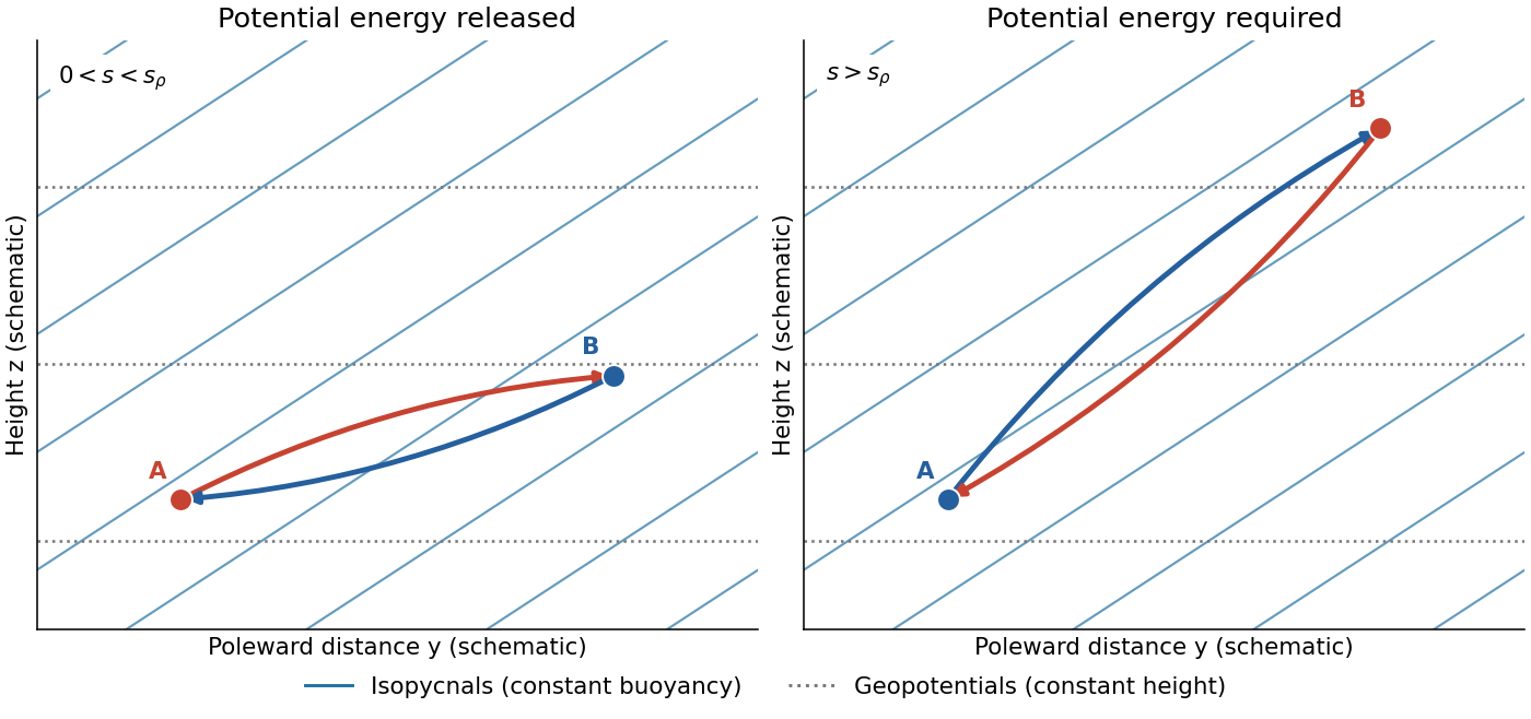
Two adiabatic parcel exchanges: a shallow poleward rise releases potential energy, whereas a rise steeper than the isopycnals costs it. Slopes are exaggerated.
Details. 
This is an energetic possibility argument for baroclinic instability, not a sufficient normal mode instability criterion. In particular, unrestricted parcel motion must not be assumed in a rotating fluid: conservation of angular momentum can impose an additional restoring effect. Symmetric instability has a separate Ertel potential vorticity criterion; ordinary Eady instability can occur without violating that criterion.
Let denote the actual horizontal velocity field. With constant nonzero Coriolis parameter , geostrophic balance and hydrostatic balance, using pressure per reference density , giveDifferentiate the first equation in to obtain thermal-wind balance:Taking the dot product with provesThus the horizontal velocity is tangent to the horizontal buoyancy contours at every height. For a fluid whose thermal equation of state makes horizontal buoyancy contours coincide with horizontal temperature contours, there is no horizontal advection across those contours. In a dry terrestrial atmosphere, use potential temperature as the materially conserved thermal variable. A salinity contribution to buoyancy would require separate treatment before interpreting the result as a statement about temperature.
The usual statement about net meridional heat transport also follows explicitly. Introduce a horizontal streamfunction such that . Integration of thermal-wind balance givesand henceFor a zonally periodic function , or vanishing endpoint contributions, the zonal integral is zero. Likewise, the anomalous eddy buoyancy flux isThe required correlation between meridional velocity and thermal anomaly is absent. A nonzero vertical phase tilt, as in the next part, permits that correlation.
Qualification of the wording. The result does not say that the local heat flux vector vanishes, or that an arbitrary open-domain integral vanishes without boundary conditions. For a concrete counterexample to that literal reading, take and . These satisfy the displayed thermal-wind balance, but is generally nonzero. What the hypotheses alone guarantee is zero transport across horizontal buoyancy contours; the vanishing zonally integrated heat transport uses the stated endpoint condition.
Take eastward , upward , positive wavenumbers , and a real instantaneous amplitude . A common growing factor does not affect the phase geometry. Put and , using the hyperbolic cosine and hyperbolic sine. The prescribed streamfunction iswhereFollowing a fixed phase givesTherefore the streamfunction pattern tilts westward with height. The lower boundary leads the upper boundary eastward.
In the conventional quasi-geostrophic streamfunction normalization, hydrostatic balance gives . ThereforeFor the phase calculation, multiplication by the constant is immaterial. Define a continuous phase ; this avoids a spurious discontinuity at . ThenThe buoyancy perturbation pattern tilts eastward with height, opposite to the streamfunction pattern. At , while , so the two fields are a quarter wavelength apart there.
Both perturbation amplitudes are largest at the boundaries. Indeed,which increase with . The physical reason is particularly clear through stratified quasi-geostrophic inversion: the Eady model has no interior background potential-vorticity gradient, and a growing normal mode has zero interior potential vorticity anomaly. The independent thermal anomalies reside at the rigid upper and lower boundaries, where meridional motion advects the basic horizontal buoyancy gradient. Each Eady edge wave induces an interior balanced flow that decays away from its boundary on scale . Their interacting, phase-locked combination produces the growing baroclinic instability. Boundary confinement of the thermal sources, rather than a rigid-wall requirement , explains the amplitude pattern.
For a sketch with a quarter-wavelength difference between the boundary streamfunction patterns, chooseAn upper positive streamfunction crest is then west of its lower counterpart, where . The buoyancy perturbation crests slope the other way. The quarter-wavelength boundary assumption is used for the streamfunction; differentiating in fixes the buoyancy perturbation and does not generally give it the same boundary phase separation.
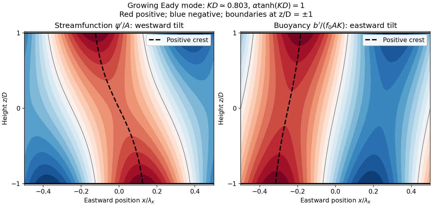
Original Eady model sketch: streamfunction crests tilt westward and buoyancy perturbation crests eastward. Dashed curves follow positive maxima; the streamfunction boundary phase difference is a quarter wavelength.
Details. 
The connection to poleward heat transport can be checked without relying on the sketch. The meridional geostrophic flow and buoyancy perturbation areAverage over one zonal wavelength, using equal averages for squared sine and cosine and zero for their product:In the Northern Hemisphere this is positive: warm anomalies preferentially move northward and cold anomalies southward. For the same eastward-increasing basic thermal wind in the Southern Hemisphere, and the basic buoyancy gradient reverses; the negative northward eddy buoyancy flux is again poleward. For thermal expansion coefficient and specific heat capacity at constant pressure , the corresponding sensible heat flux in a thermal Boussinesq approximation is . The growing amplitude makes this flux grow as . The tilt supplies the correlation absent in an untilted disturbance and reduces the background available potential energy.
The low-latitude regions of Earth absorb more incoming solar radiation than they emit as outgoing thermal radiation, whereas high latitudes have a net annual radiation deficit. The obliquity of solar incidence and the distribution of daylight create a strong latitude dependence of absorbed solar energy; emitted thermal radiation varies less strongly because terrestrial temperature contrasts are smaller. The terrestrial atmosphere and ocean therefore carry energy from the tropical surplus toward the polar deficits. Otherwise the low latitudes would keep warming and the high latitudes cooling until a different local radiative equilibrium was reached.
For a steady, zonally averaged energy balance, let be net downward radiation at the top of the terrestrial atmosphere and the total northward energy transport across latitude . A narrow spherical band and conservation of energy giveThe poleward direction is northward in the Northern Hemisphere and southward in the Southern Hemisphere. Seasonal internal energy storage modifies the instantaneous balance, but not the annual need for poleward redistribution.
Several circulation structures contribute in addition to the transient eddies produced by baroclinic instability of the middle latitudes:
- The Hadley cells, mainly between the equator and about latitude, export energy in their upper poleward branches and return air equatorward near the surface. The transported quantity includes enthalpy, gravitational potential energy and latent heat; the upper and lower branches have different thermal properties. The cross-equatorial Hadley cell is especially important in the seasonal cycle.
- Quasi-stationary Rossby waves, associated with mountains and continental heating contrasts, carry heat in the extratropical terrestrial atmosphere. Their meridional velocity and temperature anomalies can have a poleward correlation. These are an additional time-mean contribution alongside travelling weather disturbances.
- The ocean gyres in tropical and subtropical basins redistribute warm water poleward in strong western boundary currents and return cooler water equatorward over broader regions. The thermal difference between the branches produces net heat transport despite little net meridional volume transport.
- The oceanic overturning circulation, including the Atlantic meridional overturning circulation, combines warm upper water moving poleward with colder deep return water. It transports substantial heat through the tropical and subtropical Atlantic toward the northern high latitudes. Wind forcing, buoyancy exchange and mixing all help maintain this global circulation.
The Brewer-Dobson circulation additionally redistributes energy in the stratosphere, with tropical ascent and extratropical descent, although most total atmospheric heat transport occurs lower down. An Eulerian mean middle-latitude Ferrel cell is thermally indirect and can oppose the poleward transport by eddies; listing every meridional circulation as a direct poleward heat carrier would be incorrect.
Use eastward , northward , pressure coordinate increasing downward, and geopotential . Horizontal derivatives are taken on an isobaric surface. The horizontal geostrophic balance and vertical hydrostatic balance arewhere is the specific gas constant of dry air and the final equality uses the ideal gas law. At fixed latitude is independent of . Cross-differentiating givesConsequently the pressure-coordinate thermal wind equations areEquivalently, . Notice the sign: increasing eastward velocity upward means decreasing eastward velocity with , and hence poleward-decreasing temperature in the Northern Hemisphere.
For the stratospheric polar vortex estimate, the original diagram must be read on its logarithmic pressure axis. Near in the winter hemisphere, adjacent wind contours suggest an increase of roughly through a pressure decade surrounding : for example, about near and near . These are coarse graphical readings, not a sounding. ThusWith and , the poleward temperature gradient is approximatelyIf the vortex edge is taken to span roughly to , its width is , givingThe estimate depends on the width assigned to the edge and the graphical vertical shear; a range of several to roughly fifteen kelvin is more justified than a precise value. The sign remains a cold winter pole in either hemisphere. The diagram does not by itself prescribe a unique pair of edge latitudes.
At low latitudes, horizontal free-atmospheric temperature gradients are usually much smaller than at the winter vortex edge. For a comparable finite wind vertical shear, the rearranged thermal-wind balance, , is consistent with weaker temperature gradients as decreases. However, geostrophic balance loses validity near the equator because the Coriolis parameter vanishes; division by cannot be used there to derive a prediction. The weak temperature gradient approximation is better motivated by rapid horizontal internal gravity wave adjustment, together with tropical convection and the Hadley cell. Thermal-wind balance describes the balanced extratropical relation and its tendency approaching the tropics; it is not a complete causal explanation of equatorial thermal uniformity.
The quasi-geostrophic potential-vorticity equation is the leading balanced form of potential-vorticity conservation for an inviscid rotating fluid with stable density stratification, small Rossby number and an adiabatic process for each fluid element. Its parent conservation law is Ertel potential vorticity conservation. Horizontal geostrophic balance, vertical hydrostatic balance, and the beta-plane approximation reduce it to advection of one scalar by the leading horizontal geostrophic flow.
One can see its origin by combining the vertical vorticity equation with the thermal equation. Set , , and . The quasi-geostrophic approximation givesHere is the buoyancy perturbation relative to the reference stable density stratification, its buoyancy frequency, and the small vertical velocity. The stretching of absolute vorticity in the first equation is offset by the change of stratification represented by the second. More precisely,The last dot product is zero because thermal-wind balance makes perpendicular to . Adding therefore yieldsThe constant has no effect on the tendency, but its inclusion makes the connection with absolute vorticity clear. Vertical advection of is beyond the retained order; the vertical velocity has already supplied the stretching and thermodynamic terms.
- Use observed pressure or geopotential and temperature to construct a balanced initial quasi-geostrophic streamfunction, its interior potential vorticity, and the upper and lower boundary buoyancy.
- Evolve with for a small time step. For flat rigid boundaries, also evolve their thermal data with there. Appropriate lateral boundary conditions and any known large-scale circulation must accompany these fields.
- Recover the new streamfunction by stratified quasi-geostrophic inversion:
Interior potential vorticity alone is insufficient: boundary thermal anomalies can induce flow even with zero interior anomaly, as in the Eady model. The method filters fast inertia-gravity waves and is useful for large-scale extratropical weather, while tropical dynamics, convection, moisture, friction and diabatic heating require additional physics. If vertical motion is wanted, the quasi-geostrophic omega equation supplies a further diagnostic calculation.
For the proposed plane wave, define the positive squared effective wavenumberThe horizontal Laplacian contributes and the vertical stretching operator contributes . Substitution in the Linear Rossby-wave equation therefore givesThe intrinsic phase velocity is westward for positive . A stationary disturbance with and must have its westward intrinsic phase velocity exactly cancelled by the eastward background current. Solving for the squared vertical wavenumber yieldsFor Earth, with northward , in both hemispheres away from the poles. Thus an oscillatory vertical structure requiresThe background flow must be eastward but not too strong for the chosen horizontal scale. Long horizontal wavelengths have the largest allowed speed. An easterly current, , gives and an evanescent wave; so does an eastward current exceeding the upper bound. At equality and the vertical group velocity vanishes. A zonally uniform disturbance, , is a degenerate stationary pattern with no vertical Rossby wave energy propagation, so it cannot be obtained by cancelling in the preceding calculation.
A real alone does not select upward propagation. Differentiate the dispersion relation at fixed to obtain the vertical group velocity:The outgoing radiation condition for a surface source requiresFor the convention , take . The stationary phase lines then obey : they tilt westward with height while wave energy travels upward. The real conjugate component describes the same physical upward-propagating wave.
The figure suggests a winter extratropical path from the lower terrestrial atmosphere into the stratosphere, where the mean zonal flow is eastward. The summer stratosphere has westward flow and blocks such stationary Rossby waves in this idealization. A zero-wind surface is a stationary-wave critical layer in a shear flow; it also bounds the winter westerlies aloft near the upper part of the diagram. For a slowly varying real wind profile, local propagation needs along the path, sufficient surface forcing, and no intervening absorbing critical layer in a shear flow. A layer where the eastward wind becomes too strong is a turning barrier for the given horizontal wavenumbers. The uniform-current result is a local guide, not a complete prediction through a sheared spherical terrestrial atmosphere.
For scale, at latitude . A planetary zonal wavenumber has local . Taking gives the most permissive limitThe resulting limits are approximately , and for . Therefore the long planetary waves are favored; the strong core of the winter vortex can exclude shorter ones even though it is westerly. Nonzero meridional wavenumber lowers these limits further. A compressible log-pressure coordinate model would also contain a density-scale-height correction; it is absent from the equation supplied here and should not be silently inserted.
Interchanging the Northern and Southern Hemispheres changes the sign of , but only enters the dispersion relation and vertical group velocity. With the same eastward and northward , stays positive. Thus the propagation criterion is the same in both hemispheres: it selects the winter westerlies, irrespective of which hemisphere is winter. Actual amplitudes can differ because mountains, land-sea contrasts, forcing spectra and mean winds differ between hemispheres; those source differences do not reverse this propagation criterion.
Articles by others on the same topic
There are currently no matching articles.