Past exam of the kinetic theory course of the University of Oxford / 2023 (A15089W1)

Source PDF: mmathphys.web.ox.ac.uk/sitefiles/kinetic-theory-2023.pdf

Solutions to all three questions of the examination held on 12 January 2023. The cover also says Hilary Term 2022; the examination date and source filename determine the year used here. The numbered headings identify source parts without reproducing the questions. Corrections to printed formulas are explained where they arise.

Write $K_{ij}=K({\mathbf{x}}_i,{\mathbf{x}}_j)$ and $\mathbf{P}={\sum }_i{\mathbf{v}}_i$. The unit particle masses make this sum the total momentum. Exchange the two indices and use the symmetry $K_{ij}=K_{ji}$:Thus every interacting pair transfers equal and opposite momentum, even though the velocity alignment dissipates kinetic energy.

For the total kinetic energy $E_N=\frac{1}{2}{\sum }_i|{\mathbf{v}}_i{|}^2$, apply the same exchange of indices:The dissipated kinetic energy is that of relative motion. Since the total momentum is constant, $E_N-|\mathbf{P}{|}^2/(2N)=\frac{1}{2}{\sum }_i|{\mathbf{v}}_i-\mathbf{P}/N{|}^2$ also decreases. Equality holds when every pair with $K_{ij}>0$ has the same velocity; the hypotheses permit disconnected interacting groups, so they alone do not guarantee eventual global velocity alignment.

Let ${\mathbf{A}}_i={\sum }_{j\ne i}{K}_{ij}({\mathbf{v}}_j-{\mathbf{v}}_i)$. Conservation of probability in the full phase space gives the dissipative Liouville equationNormalize $\int \varrho {\prod }_i{d}^3{x}_i{d}^3{v}_i=1$. Decay at infinity makes all boundary fluxes vanish, so the equation preserves this normalization of a probability distribution.

Unlike the Hamiltonian Liouville equation, this transport has nonzero phase-space divergence. In three dimensions,The probability density increases along a contracting characteristic flow map; setting its material derivative to zero would lose conservation of probability. The $j=i$ force is identically zero, including its derivative, which is why the last sums exclude it.

Put $z_i=({\mathbf{x}}_i,{\mathbf{v}}_i)$ and $d{z}_i=d^3{x}_i{d}^3{v}_i$. Indistinguishability gives an exchangeable ensemble. Define unit-normalized marginal distributionsIntegrating the dissipative Liouville equation over $z_2,\dots ,z_N$ removes their boundary fluxes. The $N-1$ identical pair terms remain:This is the first equation of a BBGKY hierarchy, with no independence assumed yet.

The additional physical assumption is a mean-field closure for velocity alignment: neglect pair correlations, $p_2(z,z_{\star },t)\simeq p_1(z,t)p_1(z_{\star },t)$. Initial independence alone does not make this exact at later times, because the particles interact. In the usual number convention, $f=N{p}_1$ and the two-particle distribution function is $f_2=N(N-1)p_2$. Consequently the closed equation at finite $N$ isNeglecting the relative $1/N$ correction gives the intended mean-field alignment equation:Equivalently, the closure $f_2\simeq f{f}_{\star }$ incorporates this large-$N$ approximation. It cannot be an exact finite-$N$ identity with $\int f=N$, since $\int f_{2}d{z}_{\star }=(N-1)f$ whereas $\int f{f}_{\star }d{z}_{\star }=Nf$.

There is also a consistent finite-$N$ convention yielding the boxed equation directly under the independence closure: define $\tilde{f}=(N-1)p_1$ instead. Its total normalization of a probability distribution is $N-1$, rather than the physical particle number $N$. Thus the displayed source equation needs a stated normalization of a probability distribution convention, or the large-$N$ approximation, in addition to neglect of correlations. In the remaining parts we use the displayed mean-field alignment equation itself; its moment identities do not depend on the total normalization of a probability distribution.

Use $dz=d^{3}x{d}^{3}v$ and setFor unit particle mass, $\rho$ is both the number density and the mass density in the number convention of c. A fixed reference scale inside the logarithm changes $\mathcal{H}$ by a constant multiple of the conserved total mass, leaving its derivative unchanged.

Both prefactors in the source's part (d) need correction. Multiplication of the mean-field alignment equation by $|\mathbf{v}{|}^2/2$ and integration by parts givesExchange $z$ and $z_{\star }$, use the symmetry of $K$, and average the two expressions:The printed right-hand side omits $1/2$. This corrected velocity-alignment energy dissipation agrees with the pair-counting calculation in a.

For velocity-alignment entropy production, let $A(\mathbf{x},t)=\int K(\mathbf{x},{\mathbf{x}}_{\star })\rho ({\mathbf{x}}_{\star },t)d^3{x}_{\star }$. The velocity-space divergence is ${\nabla }_{\mathbf{v}}\cdot \mathbf{L}[f]=-3A$. Assuming $f>0$ and sufficient decay, integration by parts yieldsThe printed formula omits the factor $3$ from the three velocity components. In $d$ spatial dimensions, that factor would be $d$. Zeros of $f$ can be treated by a regularized entropy calculation when the required integrability holds.

A concrete smooth counterexample to both printed coefficients is $K\equiv 1$ and $f(z,0)=g(\mathbf{x})(2\pi {)}^{-3/2}{e}^{-|\mathbf{v}{|}^2/2}$, where $g$ is a positive normalized Gaussian distribution. The total mass is one, the total momentum is zero, and $\mathbf{L}[f]=-\mathbf{v}$ initially. The kinetic energy derivative is $-\int |\mathbf{v}{|}^{2}fdz=-3$, whereas the printed formula gives $-6$. The entropy functional derivative is $3$, whereas the printed formula gives $1$.

The signs describe cooling of relative velocities and contraction in phase space: $\mathcal{H}$ increases, so the fine-grained Gibbs entropy $-\mathcal{H}$ decreases. These dissipative particle dynamics are not an isolated Hamiltonian system; there is no contradiction with Liouville's theorem or the Boltzmann equation's usual entropy increase. The microscopic mechanism removing kinetic energy is outside this alignment model.

Define the local mean velocity and momentum flux byHere $\rho =\int f{d}^{3}v$ and $\mathbf{u}$ is defined where $\rho >0$. The pressure tensor separates random motion from the bulk velocity:Integrating the mean-field alignment equation over velocity space removes the force divergence and gives the continuity equationIts first velocity moment follows by multiplying by $v_i$ and using $\int v_i{\partial }_{v_j}(f{L}_j)d^{3}v=-\int f{L}_i{d}^{3}v$:Inserting the mean-field alignment equation's force and integrating each particle velocity separately givesThe right-hand side exchanges momentum between positions and aligns their bulk velocities. Its spatial integral vanishes by exchange symmetry, recovering total momentum conservation. No closure for the pressure tensor is needed for these exact velocity moment identities.

The step in the source must be at zero. We use the Heaviside step function $H(x)=1$ for $x>0$, zero for $x<0$, with its value at zero immaterial here. The printed threshold $1$ is inconsistent with both $H^{\prime }=\delta (x)$ and the stated number density. For example, measuring velocities in fixed units and taking $v_F=2$, the literal printed cutoff fills only $v<1$ and gives one eighth of the stated number density. Its distributional derivative is $\delta (x-1)$, not $\delta (x)$. The zero-threshold convention restores the stated Fermi sphere and its normalization of a probability distribution.

Let $k=|\mathbf{k}|>0$, choose $u=\mathbf{v}\cdot \mathbf{k}/k$, and abbreviate $V_{\alpha }=v_{\mathrm{F}\alpha }$. The three-dimensional phase-space distribution function is $f_{0\alpha }=C_{\alpha }{1}_{v<V_{\alpha }}$, whereIntegrate over the transverse velocity disk to obtain the parallel marginal distributionThere are no edge Dirac delta functions in $F_{\alpha }^{\prime }$ because $F_{\alpha }$ itself vanishes continuously at the endpoints. In particular, the three-dimensional constant occupation does not imply a constant parallel marginal distribution.

Use time dependence $e^{pt+i\mathbf{k}\cdot \mathbf{x}}$, with $p=\gamma -i\omega$ and $\gamma <0$ for damping. The given dielectric function becomesThe Landau contour supplies causal continuation. For a real phase velocity $a=\omega /k>V_{\alpha }$, there is no resonant pole in the populated interval, andHence this species contributes

For comparable species number densities and fixed charge ratios, $m_e\ll m_i$ implies $V_i/V_e=O(m_e/m_i)$ and ${\omega }_{\mathrm{p}i}^2/{\omega }_{\mathrm{p}e}^2=O(m_e/m_i)$. Since $\omega >k{V}_e$, the ions have $s_i\gg 1$ and ${\chi }_i=-{\omega }_{\mathrm{p}i}^2/{\omega }^2+O(k^2{V}_i^2{\omega }_{\mathrm{p}i}^2/{\omega }^4)$. Their response is negligible to leading order in the mass ratio. The real dispersion relation is thereforeThis degenerate-plasma dielectric response treats a completely degenerate, nonrelativistic Fermi gas with classical particle trajectories. It does not include quantum recoil or a collision term. A finite ion response shifts the root slightly; the boxed equation is the stated leading electron approximation.

There is no Landau damping of this branch within the completely degenerate collisionless model. Its phase velocity obeys $\omega /k>V_e>V_i$, while each parallel marginal distribution vanishes outside $|u|\le V_{\alpha }$. There are no particles at the resonant velocity, and $F_{\alpha }^{\prime }(\omega /k)=0$. The Landau contour consequently contributes no imaginary part to the dielectric function; a real root is allowed with $\boxed{\gamma =0}$.

If a small nonzero temperature supplied a tail beyond the Fermi surface, the conclusion would change: the resonant derivative would generally be nonzero. For the convention $p=\gamma -i\omega$ and a simple weakly damped root, expanding the continued dielectric function would give $\gamma =-{ϵ}_I(\omega ,k)/{\partial }_{\omega }{ϵ}_R(\omega ,k)$. This conditional formula is not needed to manufacture damping for the exact cutoff. Neither collisional attenuation nor nonlinear evolution is included in the given dispersion relation.

Let $\kappa =k{V}_e/{\omega }_{\mathrm{p}e}$ and $s=\omega /(k{V}_e)$. The long-wavelength electron branch has $|s|\gg 1$. The convergent power seriesturns the degenerate-plasma dielectric response intoSubstitute ${\omega }^2={\omega }_{\mathrm{p}e}^2+a{k}^2{V}_e^2+O(k^4{V}_e^4/{\omega }_{\mathrm{p}e}^2)$. The coefficient of $k^2$ is $a-3/5$, so the degenerate-plasma Langmuir dispersion isThe Langmuir wave therefore has a finite frequency at zero wavenumber, with the first dispersive correction set by the Fermi velocity. Indeed the occupied Fermi sphere has $⟨v_{\parallel }^2⟩=V_e^2/5$, so the coefficient $3⟨v_{\parallel }^2⟩=3V_e^2/5$ agrees with the high-phase velocity velocity moment expansion.

Screening-length convention. The source defines ${\lambda }_{\mathrm{D}e}^{\mathrm{exam}}=\sqrt{3}{V}_e/{\omega }_{\mathrm{p}e}$, so its long-wavelength condition is equivalent to $\kappa \ll 1$. We retain that definition when expressing answers in its symbols. The actual electron Thomas-Fermi screening length obtained from the static response is insteadFor a concrete comparison, at $k={\omega }_{\mathrm{p}e}/V_e$, the static dielectric function is $4$; using the printed length as the physical Thomas-Fermi screening length would give $1+1/3=4/3$. Calling the printed length the Debye length thus differs from the physical degenerate-electron screening convention by a factor of three. It does not affect the boxed dimensional dispersion relation.

For the positive-frequency branch write $s=1+\delta$, $\delta >0$, and $Q=k^2{V}_e^2/(3{\omega }_{\mathrm{p}e}^2)={\kappa }^2/3$. The degenerate-plasma dielectric response is equivalent toAt large $Q$, a logarithmic divergence is needed to balance the right-hand side; hence $\delta \ll 1$. Keeping the constant as well as the large term givesMore precisely the relative correction is $O((1+Q)e^{-2(1+Q)})$. The additive constant $-2$ in the exponent fixes the leading prefactor $2e^{-2}$ and should not be discarded.

The negative-frequency branch follows from the even real dielectric function outside the occupied interval. ThusUsing the physical Thomas-Fermi screening length instead gives $\delta \sim 2e^{-2-2(k{\lambda }_{\mathrm{TF}}{)}^2}$. This is degenerate-plasma zero-point sound: the phase velocity lies exponentially close to, but strictly beyond, the edge of the Fermi sphere for every finite $k$ in this approximation. The limit is a property of the supplied classical-trajectory kinetic theory; applying it at microscopic wavelengths would require checking quantum recoil, which that equation omits.

The two real branches start at $\omega =\pm {\omega }_{\mathrm{p}e}$, have zero initial slope, and approach the lines $\omega =\pm k{V}_e$ from outside the populated parallel-velocity region. The original plot solves the degenerate-plasma dielectric response numerically; the shaded wedge shows where particles with resonant parallel velocities exist.

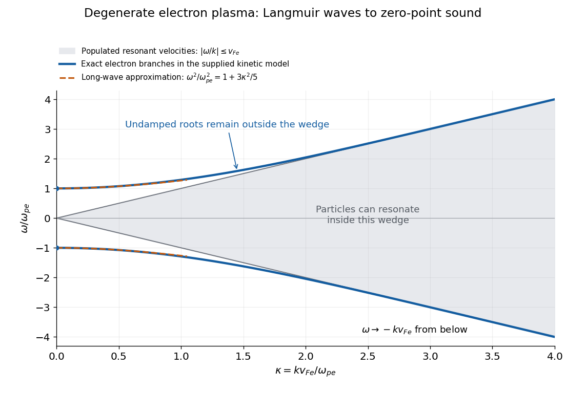
The distinction from a nondegenerate gas with a Maxwellian Maxwell-Boltzmann velocity distribution is its tail. A Maxwellian has resonant particles at every finite phase velocity. Its long-wavelength Langmuir waves have exponentially weak Landau damping, but at shorter wavelengths that damping becomes strong. The ideal degenerate cutoff instead permits this undamped branch to persist continuously into degenerate-plasma zero-point sound. The coefficient $3V_e^2/5$ in c is also different from the classical thermal dispersive coefficient.

A natural additional branch is a degenerate ion-acoustic wave. For singly charged ions with equal electron and ion number densities, degenerate electron pressure supplies a restoring force while ion mass supplies inertia. The electron equation of state has $d{P}_e/d{n}_e=m_e{V}_e^2/3$, suggesting, at long wavelengths,Both species are degenerate here, so $V_i=(m_e/m_i)V_e$. The hierarchy $V_i\ll c_s\ll V_e$ explains the damping: there are no resonant ions, but there are resonant electrons inside their parallel marginal distribution. That electron marginal distribution has a small nonzero slope at $u=c_s$, even though the full three-dimensional occupation is constant inside the Fermi sphere. One therefore expects weak electron Landau damping, of relative order $\sqrt{m_e/m_i}$, rather than exact absence of damping. Ion degeneracy pressure adds a relatively small correction to $c_s^2$. This reasoning concerns an electrostatic ion-acoustic wave; transverse or magnetized branches require additional field dynamics or a background magnetic field.

The action-angle variables $(\mathbf{\theta },\mathbf{J})$ are canonical coordinates, with $[{\theta }_a,J_b]={\delta }_{ab}$. In the convention $\dot{g}={\partial }_{t}g+[g,H]$, their Poisson bracket isIn particular, Hamilton's equations read $\dot{\mathbf{\theta }}={\partial }_{\mathbf{J}}H$ and $\dot{\mathbf{J}}=-{\partial }_{\mathbf{\theta }}H$, fixing the sign needed below.

Define the unperturbed orbital angular frequency vector byIt is the rate of advance of the angle variables along the unperturbed Hamiltonian flow; the action variables are constant. Expand the Collisionless Boltzmann equation to first order in the perturbations. Since $f_0$ and $H_0$ depend only on the action variables, $[f_0,H_0]=0$, andThe omitted Poisson bracket $[\delta f,\delta \Phi ]$ is quadratic in the perturbations. Use the Fourier series conventionFor each harmonic the linear ordinary differential equation isMultiplication by the integrating factor $e^{i\mathbf{k}\cdot \mathbf{\Omega }t}$ and use of $\delta f_{\mathbf{k}}(0)=0$ give the causal linear response in action-angle variables:The zero harmonic stays zero at this order. This formula retains the entire forcing history; replacing it immediately by a resonant Dirac delta function would discard the transient response.

Since $L_z=J_{\varphi }$, Hamilton's equations giveFor the spherical unperturbed Hamiltonian, $H_0=H_0(J_r,L)$; in these particular action-angle variables the third component ${\Omega }_{\varphi }=0$ describes the fixed orientation of the orbital plane. It should not be confused with the physical azimuthal angular velocity of a particle around its orbit.

The conserved normalization of a probability distribution $\int f{d}^3\theta d^{3}J=1$ makes the expected value of specific angular momentum equal to $\int L_{z}f{d}^3\theta d^{3}J$. Its time derivative is the torque per unit halo mass:This follows either by averaging the single-particle equation or by integrating the Collisionless Boltzmann equation against $L_z$, with vanishing boundary fluxes.

The term $f_0{\partial }_{{\theta }_{\varphi }}\delta \Phi$ integrates to zero over the periodic angle variable. Thus the first nonzero torque is quadratic in the perturbation. Use the Fourier series expansions of b; the source's reference here to part (a) is a numbering slip. Integrating the product over all three angle variables yieldsReality of the potential energy per unit mass gives $\delta {\Phi }_{-\mathbf{k}}=\delta {\Phi }_{\mathbf{k}}^{\ast }$; likewise $\delta f_{-\mathbf{k}}=\delta f_{\mathbf{k}}^{\ast }$. Conjugate harmonics make the total torque real. The sum is over all integer vectors, so no extra factor of two should be inserted.

Write $m=k_{\varphi }$, $B_{\mathbf{k}}=\mathbf{k}\cdot {\partial }_{\mathbf{J}}{f}_0$, and let the detuning from the rotating perturbation beSubstitute $\delta {\Phi }_{\mathbf{k}}={\Psi }_{\mathbf{k}}{e}^{-im{\Omega }_{\mathrm{p}}t}$ into the linear response in action-angle variables, then set $\tau =t-t^{\prime }$:At exact resonance the last quotient is interpreted by its continuous limit $it$. Inserting this response in c givesPair $\mathbf{k}$ with $-\mathbf{k}$. Because $B_{-\mathbf{k}}=-B_{\mathbf{k}}$, ${\Delta }_{-\mathbf{k}}=-{\Delta }_{\mathbf{k}}$, and $|{\Psi }_{-\mathbf{k}}{|}^2=|{\Psi }_{\mathbf{k}}{|}^2$, the imaginary cosine terms cancel. The finite-time torque isThis is a leading, second-order response in the perturbation amplitude.

For the long-time limit, assume a continuum of occupied action variables, sufficiently smooth integrable weights, convergent harmonic sums, and regular resonance surfaces ${\nabla }_{\mathbf{J}}{\Delta }_{\mathbf{k}}\ne 0$ wherever a contributing surface intersects the distribution. Assume also that the perturbation is weak enough to neglect nonlinear trapping and secular changes in $f_0$, and that the prescribed stellar bar pattern and its coefficients stay fixed. Then phase mixing removes nonresonant transients in the integrated response. The relevant long-time resonance kernel is the distributional convergenceIt is not a pointwise limit: at $x=0$ the kernel equals $t$. To justify its use under the integral over action variables, resolve the integral into detuning surfaces; the coarea formula givesSmoothness and decay of this surface weight reduce the limit to the one-dimensional long-time resonance kernel. Equivalently, a causal convergence factor $e^{-\eta \tau }$ gives $\mathrm{Re}{\int }_0^{\infty }{e}^{-\eta \tau -i\Delta \tau }d\tau =\eta /({\eta }^2+{\Delta }^2)\to \pi \delta (\Delta )$ as $\eta \downarrow 0$.

Therefore the resonant torque from a rotating perturbation isOnly orbital resonances contribute to this steady integrated torque. The limit is a formal weak-perturbation limit, or an intermediate-time approximation after phase mixing but before substantial secular redistribution. It does not prove an unchanged halo can absorb angular momentum at this rate forever. A discrete set of orbital frequencies, singular resonance surfaces, or strong trapping can invalidate the stated steady limit.

Apply the chain rule to $f_0=f_0(E)$ with $E=H_0(\mathbf{J})$:On the resonance selected by the Dirac delta function, $\mathbf{k}\cdot \mathbf{\Omega }=k_{\varphi }{\Omega }_{\mathrm{p}}$. ThusEvery weight is nonnegative, and $-f_0^{\prime }(E)>0$. Strict positivity additionally requires a populated nonaxisymmetric resonance with nonzero coupling on a set of positive surface measure. The unconditional statement is nonnegativity, rather than positive definiteness. As a concrete counterexample to strict positivity of this formula, retain one nonzero conjugate harmonic pair with $k_{\varphi }\ne 0$ and choose its smooth coefficient ${\Psi }_{\mathbf{k}}$ supported in an open region $|{\Delta }_{\mathbf{k}}|>d>0$. The perturbation is nonzero but has zero resonant coupling, so $\mathcal{T}=0$ even when $f_0^{\prime }(E)<0$. The even simpler zero-perturbation case also gives zero. Whether a particular physical stellar bar has nonzero resonant overlap is additional information.

For a coupled stellar bar and halo, the halo gains positive angular momentum and exerts the opposite torque on the stellar bar. If the halo mass is $M_h$ and the rigid stellar bar has constant positive moment of inertia $I_b$, thenThis bar-halo angular-momentum transfer is a form of dynamical friction: a resonantly coupled stellar bar tends to slow down while the dark matter halo spins up. Actual long-term evolution changes both the stellar bar pattern and the halo distribution function, so the fixed-pattern response must then be updated. If the stellar bar changes its moment of inertia, the general relation is $d(I_b{\Omega }_{\mathrm{p}})/dt=-M_h\mathcal{T}$; positive moment of inertia alone would not fix the sign of $d{\Omega }_{\mathrm{p}}/dt$ without that rigidity assumption.