Original paper: Public original PDF, physical pages1–8; question pages2–8.
Use fractional coordinates in a conventional cubic cell with an atom at the origin. The diamond cubic structure consists of an FCC Bravais lattice with the two-atom basisThe FCC translations within the conventional cell are , , and . Adding the basis gives eight atoms per conventional cell. Equivalently, two identical FCC sublattices are displaced by . It is not a monatomic close-packed arrangement: every atom has four tetrahedrally arranged nearest neighbors rather than twelve.
In the projection, label each atom by its fractional height. The and columns have height0; and have height1/2. The additional four columns are and at height1/4, and and at height3/4. Boundary columns repeat periodically; they must not be counted as full extra atoms.
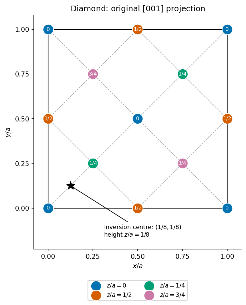
Original fractional-coordinate projection of diamond silicon, with atom heights, vertical mirror traces and a bond-centred inversion point
. Details. 
The vertical mirrors of the diamond cubic structure have the required orientation: their normals lie in the plane. In the chosen atomic-origin convention, their traces satisfywith expressed as fractions of . These are the two orientations of vertical mirrors and their translated copies. For example, the plane interchanges the first two coordinates and leaves every diamond site in an equivalent site. Reflection in sends to , which also preserves the full three-dimensional motif.
The projected traces alone do not test a mirror: the atom heights must also agree under reflection. In particular, a vertical trace can appear plausible in an unlabelled projection but does not preserve all heights as a pure mirror; glide operations are different symmetry elements.
Bond-centred inversion in diamond cubic gives one inversion centre at the midpoint of a nearest-neighbor bond:Mark its projected point and label its height . Inversion about this point sends to . It exchanges the two identical FCC sublattices and therefore preserves the crystal. An individual atom at the chosen origin is not an inversion centre.
The nearest-neighbor displacement is , of length . Touching hard spheres therefore obeyThere are eight atoms per conventional cubic cell, givingFor monatomic FCC close packing, four atoms per cell touch along a face diagonal, so andThus the diamond packing fraction is much smaller. The tetrahedral network leaves substantial open volume. Although its Bravais lattice is FCC, the two-atom motif and the shorter hard-sphere contact distance prevent it from inheriting the FCC close-packing fraction.
The four FCC translations give a lattice structure factor that is nonzero only when are all even or all odd. The identical two-atom motif then multiplies it byFor the FCC part is allowed, but the motif factor is . HenceIn the projection, equal numbers of atoms occur at . Their phases are respectively . The paired layers cancel exactly for equal silicon scattering amplitudes. This diamond-basis diffraction extinction is additional to the FCC centring rule; it is not evidence that no atoms lie on the nominal reflecting planes.
For indexing a diamond-cubic powder pattern, and Bragg's law gives . Using half of each printed scattering angle, the ratios to the first peak are approximatelyMultiplying by3 gives the allowed sequence . ThusThe numerical calculation, expressed without assuming a historical Data Book wavelength, isTherefore . As a separately identified reference convention, choosing Cu K with givesThat wavelength follows from the copper transition near in the NIST transition database, using .[ref]
X-Ray Transition Energies Database by National Institute of Standards and Technology. Copper, experimental KL3 transition energy
The paper says Cu K but does not give the line-selection convention or an explicit wavelength. A rounded unresolved-doublet wavelength, for example , would instead give about . These are conditional wavelength evaluations, not claims about the unavailable historical Data Book. The angles are internally consistent with one cubic parameter; they should not be replaced by literature peak positions simply to obtain a familiar silicon value.
The normal to the section is , so its in-plane principal vibration directions are and . Their refractive-index difference isThe slow direction is . The optical path retardation isAt an angle between a principal direction and the polarizer, ideal crossed-polar transmission has the formwhere is the intensity after the first polarizer. The two components recombine parallel to the incident polarization when , and the crossed analyser removes them. ConsequentlyThe next order is260nm, outside ordinary visible illumination. At exact principal-axis alignment, and every wavelength is extinguished, explaining the black appearance rather than a special single-wavelength cancellation.
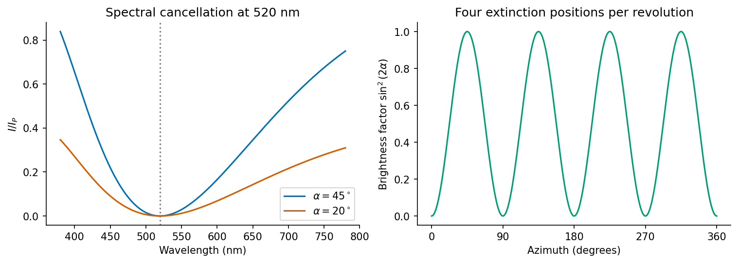
Original crossed-polar transmission calculation for the given retardation, including the visible extinction wavelength and azimuthal brightness factor
. Details. 
An unstressed glass is optically isotropic, so it does not split incident light into differently phased in-plane components; it remains dark between crossed polars. A natural explanation of the colored regions after heating is devitrification: anisotropic crystallites have nucleated in the glass. Edges and surfaces provide heterogeneous nucleation sites, making their greater concentration there plausible.
Each approximately uniform crystallite can give a nearly uniform interference colour. Regions with similar thickness and effective birefringence have similar retardation and therefore similar spectral colour, while differing azimuths multiply the intensity by and change brightness. Identical hue does not prove identical three-dimensional crystallographic orientation.
Stress-induced birefringence is a possible alternative in a heat-treated glass. The observations alone do not uniquely prove crystallinity; rotating-stage extinction, morphology or diffraction could distinguish the explanations. The crystallite interpretation is the straightforward phase-transformation explanation, without inventing a composition or heat-treatment schedule.
On rotating a fixed crystallite around the microscope axis, the angle to the fixed polarizer changes. The factor repeats every90degrees. Each birefringent region is therefore extinguished four times in a complete revolution and reaches maximum brightness45degrees from its own extinction positions.
Different regions need not extinguish together if their principal in-plane directions differ. For a fixed propagation direction through a uniform region, azimuthal rotation changes brightness more directly than its retardation colour: the underlying index difference and thickness remain the same. The isotropic unstressed matrix remains dark throughout rotation.
The quartz compensator is a birefringent optical compensator: a retarder of known principal directions. With its principal axes at45degrees to the polarizer and analyser, the previously dark isotropic background acquires the compensator's own interference colour. The crystals are now viewed through two retarders.
When a specimen's slow axis is parallel to the compensator's slow axis, the retardations add. A90degree relative principal-axis rotation pairs the specimen's slow axis with the compensator's fast axis, and the signed retardations subtract:Thus different crystallites can shift to higher or lower interference orders even if their original hue was similar. In the subtracting orientation, equal magnitudes can compensate and yield extinction. These shifts identify fast and slow specimen directions.
At a general relative angle the full polarization transformation is required; simple scalar addition is only valid for aligned principal axes. The source does not specify the compensator retardation, so no unique list of resulting named colours can be assigned. The robust predictions are a changed background, orientation-dependent addition or subtraction, and possible compensation.
The materials interpretation is a cooling-rate gradient in a near-eutectoid steel. Before transformation, the parent thermodynamic phase is austenite. A small section can cool rapidly enough to suppress diffusional decomposition and form martensite, a supersaturated, highly strained transformation product. A much thicker interior cools more slowly and can transform diffusively to pearlite: alternating ferrite and cementite lamellae grouped into colonies. Bainite or mixed products are also possible for intermediate histories.
The likely contrast is therefore a martensite-rich rapidly cooled region and a more pearlitic slowly cooled interior. Brittle fracture is promoted by the highly strained martensitic state, residual stresses and local stress concentration. A larger intact interior need not share the same microstructure or local loading. The observations are consistent with this contrast, not a measurement proving pure thermodynamic phases everywhere.
The sketches below are generic steel microstructures, rather than a component design or fabrication prescription. No cooling curve, dimensions or transformation diagram is provided, so exact thermodynamic phase fractions, plate sizes and a universally pearlitic centre cannot be inferred.
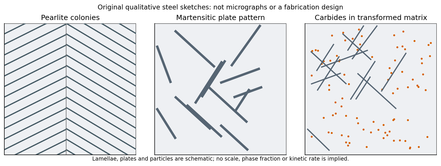
Original qualitative steel microstructure sketches: lamellar pearlite, a strained martensitic plate structure and carbide precipitation within a transformed matrix
. Details. 
In tempered martensite, the metastable carbon-supersaturated martensitic matrix can evolve toward a lower-carbon ferritic matrix containing fine carbides. Carbon segregation and precipitation reduce supersaturation and tetragonal lattice distortion; recovery can reduce internal strain while the original plate or lath pattern remains recognizable. This is tempering, rather than a fresh austenite-to-pearlite transformation.[ref]
Tempered Martensite by H. K. D. H. Bhadeshia. Introduction and Virgin Microstructure, carbon redistribution and retained plate structure
A generic sketch consequently replaces a uniform highly strained plate interior by a lower-carbon matrix with dispersed carbide particles, as in the third panel above. This provides a qualitative materials explanation for a changed fracture response. It does not specify a manufacturing optimization, and tempering is not a guarantee of monotonic toughness improvement in every steel: carbide morphology, impurities and retained austenite matter. The source reports the observed outcome, so the explanation must not be turned into a universal process recommendation.
Use the supplied Arrhenius law as a diffusion-scale calculation. The stated temperature and duration become and . With ,With the standard diffusion-distance convention, the characteristic scale isThe one-dimensional rms displacement is about30micrometres, and the three-dimensional rms displacement about53micrometres. These different prefactors follow from the diffusion-distance convention; the diffusion coefficient is unchanged.
The scale is much larger than atomic spacing and can permit local carbon redistribution and carbide formation over microstructural distances. It is not evidence that the entire macroscopic specimen becomes compositionally homogeneous. Trapping, concentration gradients, evolving carbides and the use of a ferrite diffusivity for an initially defect-rich transformation product limit a literal tracer-distance interpretation.
TODO: Practical weapon-fabrication and optimization instructions are not provided. The general metallurgy and diffusion analysis are retained in the preceding parts; this manufacturing subpart remains explicitly limited.
For distinguishable lattice sites occupied by mutually indistinguishable atoms of each species, the number of configurations isUsing Stirling's approximation,For one mole, and , soEquiatomic configurational entropy follows when the composition has , givingThe reference is the unmixed configurational arrangement, and the model assumes random site occupation without short-range order. It counts configurational entropy, not all vibrational, electronic or magnetic entropy. A large number of elements does not by itself guarantee a stable single solid solution: competing thermodynamic phases and the enthalpy term also enter the Gibbs free energy.
A Shockley partial dislocation in an FCC slip plane has Burgers vector of the family . Its vector must lie in the specified plane, and the two vectors must sum to the perfect dislocation vector.
For ,Their sum is , and both have zero dot product with . Interchanging leading and trailing labels does not change these vector identities.
Each perfect vector has squared magnitude , whereas the sum of the two partial squared magnitudes is . The line-energy estimate proportional to therefore favors separation, opposed by the stacking-fault energy of the ribbon between the partials.
Use the two partials on each plane as obtained above. The four pairwise sums, in units of , areThe shortest resultant gives the largest line-energy reduction in the approximation:The initial summed squared magnitude is and the final value is , a sixfold reduction in that part of the energy estimate.
The line of intersection of the two original planes is parallel toIts dot product with the resultant Burgers vector is zero, so the junction is edge in character. A plane containing both line and Burgers vector has normal , rather than an FCC close-packed glide normal. The resulting stair-rod dislocation is therefore sessile for ordinary glide and can form a Lomer-Cottrell lock. It obstructs further dislocation motion and promotes work hardening.
This energetic comparison assumes comparable line lengths and elastic prefactors. Geometry, line character and stacking-fault geometry affect a complete junction-energy calculation, but the small resultant identifies the favorable candidate requested by the vector model.
The original diagram is a Kelvin-Voigt model: a spring and a dashpot act in parallel. The spring is an ideal elastic element, ; under its own sinusoidal stress its strain is in phase with stress and energy is stored reversibly. The dashpot is viscous, ; its strain under an oscillating stress lags by90degrees and mechanical energy is dissipated.
In parallel the strain is common and the branch stresses add:For imposed harmonic stress, the strain amplitude and phase lag areThe short- and long-timescale limits follow under the printed roman labels below.
A sudden constant stress gives delayed, bounded creep:The strain is initially zero because an instantaneous change would require an infinite dashpot stress. Initially the dashpot carries the load, with finite strain rate ; the spring gradually carries more of it as the rate decays. On unloading, the strain recovers exponentially to zero. The network does not produce the instantaneous strain jump or unbounded constant-stress creep of a series Maxwell element.
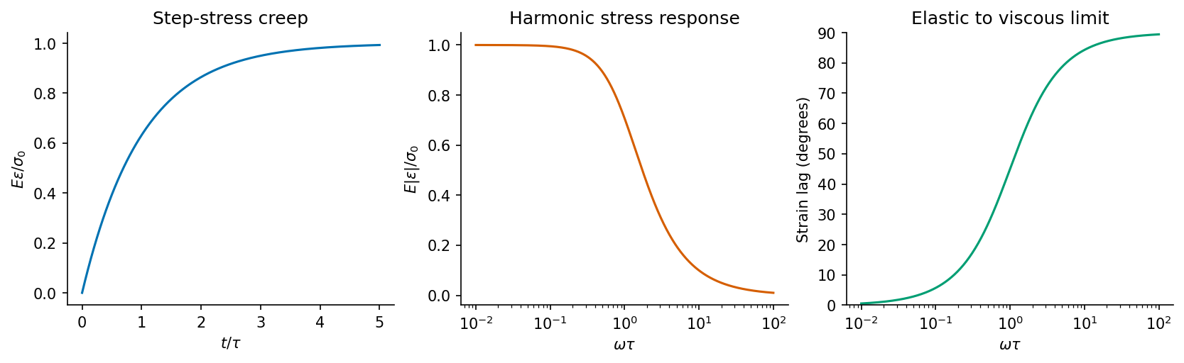
Original Kelvin-Voigt predictions for step-stress creep, frequency-dependent compliance and stress-strain phase lag
. Details. 
On a timescale short compared with , or for , the dashpot strongly resists rapid deformation. The imposed oscillating stress produces a small strain, of amplitude approximately , nearly90degrees behind the stress. The network appears stiff and predominantly viscous in this stress-controlled high-frequency limit. It is not an ideal perfectly rigid body at finite frequency.
For a slowly varying load with , the dashpot stress is small relative to the spring stress. The strain approaches almost in phase, so the low-frequency response is predominantly elastic. A constant load approaches the finite equilibrium strain ; it does not sustain steady viscous flow in this parallel network.
For a rubber-like solid, a spring is a first model of recoverable elasticity, while a viscous element can represent rate-dependent loss and delayed recovery. If the observed material has both an immediate extension and a further bounded delayed creep, a spring in series with a Kelvin-Voigt element is a simple linear-solid model:The first term is immediate and recoverable; the second is delayed and also recoverable. A single Voigt element misses the immediate compliance, while a free series dashpot would predict unbounded flow that an intact crosslinked rubber need not show.
These are local small-strain analogues. Large-strain rubber elasticity is nonlinear, nearly incompressible and sensitive to temperature, loading history and internal damage. A small set of linear springs and dashpots cannot reproduce every amplitude, timescale or hysteresis loop.
TODO: Match the model to the unavailable practical-class observations. No particular measured rubber trace, specimen state or fitted constants are supplied.
A physical mechanics model of wood must at least acknowledge anisotropy: stiffness and creep depend on loading direction. Direction-dependent elastic elements can represent different small-strain moduli, and delayed elastic branches can approximate time-dependent strain. A linear-solid network can therefore be a local fit under specified direction, moisture and temperature, rather than a universal scalar constitutive law.
If experiments show an immediate strain followed by delayed creep, a spring plus a Voigt branch can capture those features. If permanent set remains after unloading, that recoverable model is insufficient and an irreversible deformation branch or damage law is needed. Strength loss, splitting, moisture-dependent response and nonlinear compression cannot be represented by one fixed linear Voigt element.
TODO: Match the network and any irreversible branch to the unavailable practical-class observations. These are conditional materials-mechanics possibilities, not invented laboratory results. No biological structure or organism-specific mechanism is required here.
At equilibrium between two thermodynamic phases of a pure substance, their molar Gibbs free energies are equal. Along a coexistence line,Subtracting the two differentials givesFor a nonzero volume change,The second equality uses on coexistence. Total entropy and volume changes may be used instead if they refer to the same amount of material. The ratio must use one consistent transformation direction, so reversing the labels changes both signs and leaves the slope unchanged. This is the general Clapeyron equation; the ideal-vapour approximation often called Clausius-Clapeyron makes further assumptions not needed for two solids.
A multi-anvil press transmits a large external load through several hard anvils onto a confined pressure medium surrounding the sample. Reducing the loaded area raises pressure, while the surrounding medium and gasket limit lateral escape. A resistive heater within the assembly can heat the sample, with insulation and temperature sensing arranged around it. It provides relatively large sample volumes and useful bulk, high-temperature experimental conditions, but access to the sample and optical paths is restricted, pressure gradients and calibration matter, and the maximum pressure is constrained by anvil strength and geometry.
A diamond anvil cell squeezes a very small sample and pressure medium in a gasket hole between opposed diamond culets. Diamond combines high strength with useful optical transparency, permitting spectroscopy and optical pressure calibration as well as suitable X-ray access. Heating can be external or laser-based. The very small contact area permits high pressure from a modest total force, but gives a tiny sample volume. Nonhydrostatic stress, pressure gradients, gasket deformation, heating gradients, chemical compatibility and diamond failure are important limitations.
Neither device generates pressure by force alone independent of area and confinement. Nor does a nominal force-to-area ratio guarantee a known hydrostatic sample pressure; experimental pressure and temperature must be calibrated. The two assemblies trade sample volume and access against pressure reach rather than one being universally preferable.
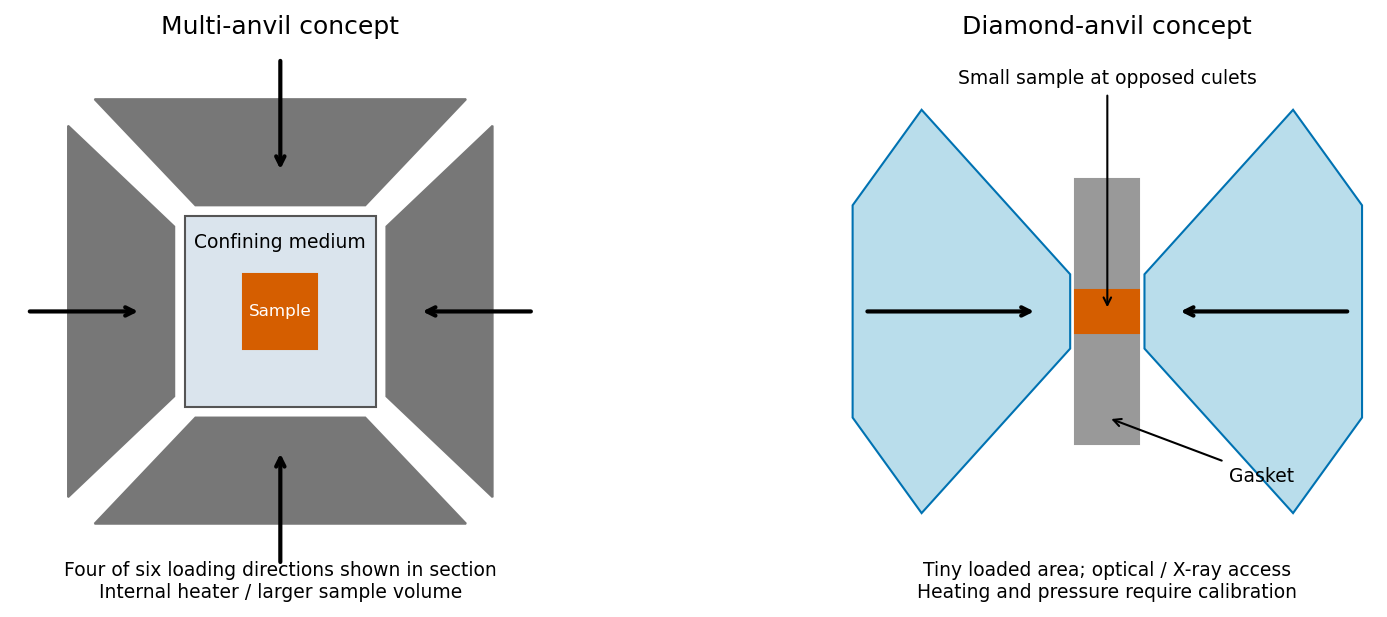
Original conceptual comparison of multi-anvil load transmission and opposed diamond culets, showing confinement and qualitative heating/access tradeoffs
. Details. 
Diamond can be metastable: its Gibbs free energy is higher than graphite's under ambient conditions, but transformation is kinetically inhibited. Conversion requires substantial rearrangement of the strong carbon-bond network and the formation and growth of a new thermodynamic phase, with an activation and nucleation barrier.
At room temperature the rate can be extremely small even though the free-energy change favors graphite. Thermodynamic stability specifies the preferred equilibrium state, not the time needed to reach it. Persistence of diamond therefore does not contradict graphite's ambient equilibrium stability.
Use the same molar amount for both thermodynamic phases. A hexagonal cell built from two basal lattice vectors at120degrees has volume , not the volume of a three-times-larger full hexagonal prism. With four atoms per stated graphite cell,Diamond has eight atoms per conventional cubic cell, soFor graphite transforming to diamond,ThereforeThe positive slope reflects diamond's smaller entropy and volume. Higher temperature favors the higher-entropy graphite thermodynamic phase, requiring greater pressure to compensate in favor of the smaller-volume diamond thermodynamic phase.
This estimate treats the supplied ambient molar entropies and volumes as applicable near coexistence and neglects their changes through thermal expansion, compressibility and heat capacity. It gives an approximate gradient, not the transition pressure or a complete high-pressure thermodynamic phase boundary; an intercept would require an additional free-energy datum.
At two-phase equilibrium, the endpoints of a common tangent to the two molar free-energy curves give the coexisting compositions. They are not the separate curve minima. Reading the graph gives approximately and , with a few atomic-percent graphical uncertainty.
Let be the fraction of atoms in the precipitate thermodynamic phase. Conservation of the overall B fraction givesand henceAbout85percent remains in the B-richer matrix. Smooth readings of the original curves put the result near14–15percent; the graph does not justify many significant figures. The result is an atomic or molar thermodynamic phase fraction. Its identification with a volume fraction in the next estimate requires comparable atomic volumes of the two thermodynamic phases.
Assume the two thermodynamic phases have similar atomic volumes, so use . Model the stated average pitch by one sphere per representative cubic volume . If the sphere diameter is ,Using the more literal lever-rule reading0.145 gives about0.65micrometres instead, within graphical uncertainty. The central estimate is therefore a diameter of roughly two-thirds of a micrometre.
A random distribution does not make a nearest-neighbor mean distance exactly equal to the cube root of inverse number density. The representative cubic spacing is an explicit geometric closure, not evidence that the precipitates actually form a cubic lattice. Unequal molar volumes or a different spacing statistic would change the inferred size.
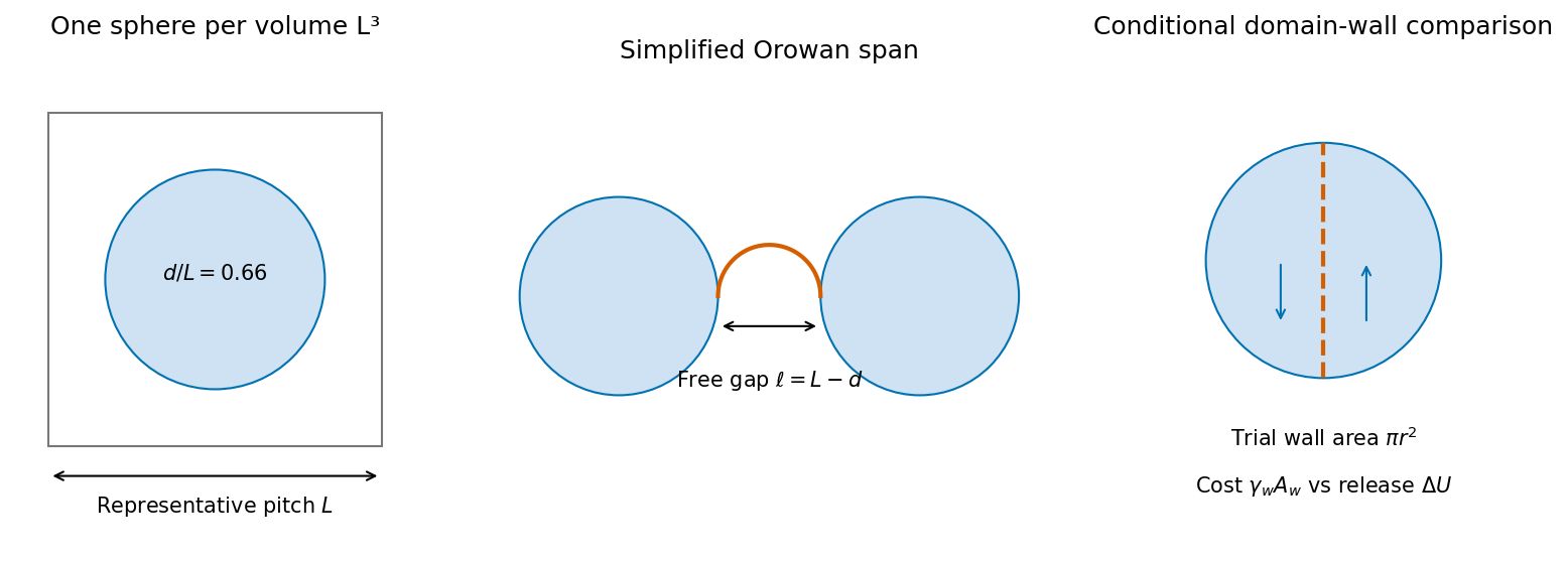
Original geometric estimates for a spherical precipitate fraction, a dislocation free gap and a trial internal domain wall
. Details. 
Orowan bypass bows a dislocation around an unshearable obstacle and leaves a loop. A dislocation line-tension estimate for a segment with tension gives the limiting shear-stress scalewhere is a free obstacle gap on the slip plane. For an FCC perfect dislocation,Using and the simple gap estimate givesConverting to tensile stress requires an orientation factor. With an explicitly assumed polycrystalline FCC Taylor factor ,The graph and spacing approximations do not justify a precise last digit. A favorably oriented single crystal with Schmid factor1/2 would instead give , around110MPa.
This is a line-tension estimate. A true slip-plane obstacle distribution, line character, logarithmic elastic corrections and precipitate size distribution are not specified. If the quoted pitch is used directly as an effective free spacing, neglecting diameter, the same simplified calculation gives and . The larger gap-corrected estimate explicitly uses the size inferred above; the tensile factor and spacing convention must not be silently treated as provided measurements.
A single-domain precipitate has no internal domain wall available to move. Magnetization changes therefore require rotation, curling or reversal of a particle's magnetization, rather than ordinary wall displacement through that particle. Relative to a larger multidomain material this can increase coercivity, but the actual coercivity depends on anisotropy, shape and particle interactions. If thermal activation over the anisotropy barrier is rapid on the observation timescale, superparamagnetic behavior can instead suppress remanence. Ferromagnetic composition plus small size alone does not prove a permanent hard magnet.
For an elementary wall-energy comparison, imagine one planar wall through a sphere of radius . Its area is . If that trial two-domain state removes essentially all of the specified stray-field energy while adding wall energy , stability of the uniform state requiresWith and the supplied ,This is the requested scale under a full stray-energy-release and one-planar-wall approximation; it is a lower-bound estimate within that model.
A more exact comparison uses the actual energy reduction of the competing domain pattern, not necessarily the whole original stray energy:No domain geometry, anisotropy energy or barrier is supplied to determine or establish that the observed state is the thermodynamic ground state rather than kinetically trapped. Thus the given information alone does not establish an unconditional positive numerical lower bound independent of the competing pattern; the elementary estimate must retain its stated assumptions.
Articles by others on the same topic
There are currently no matching articles.