For real , use logarithmic differentiation: . The product rule gives , henceWork on an interval where is defined. The positive-base condition makes the variable real power unambiguous.
Implicit differentiation gives . ThereforeFor real , the denominator is at least one, so division introduces no singularity. In fact the function is strictly increasing, consistent with a unique real branch .
The integration region lies between the line and the parabola , with . It has a portion below the -axis bounded above by , and a portion above it bounded below by . Horizontal slices change form at ; keeping that split is essential when reversing the order of integration.
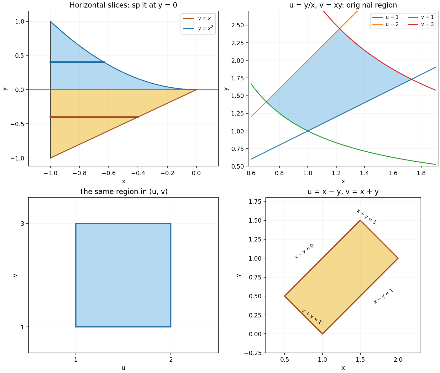
For , a horizontal slice runs from to the line . For , it runs from to the negative branch of the parabola. Thus the reversed iterated integral isThe positive branch is outside the original integration region.
In the original order of integration,In the reversed order, the below-axis contribution is , and the above-axis contribution is . Their sum is again . A negative answer is possible because the integrand changes sign; the integral is not the area of the region.
In Cartesian components, , with constant . Taking the gradient component by component givesThe constancy of matters: if it depended on position, derivatives of its components would also contribute.
The vector calculus identity gives zero because a constant vector field has zero curl and . ThusEquivalently, the Cartesian components are , and each component is independent of the coordinate used in its contribution to the divergence.
Away from the origin, the product rule and giveThe field is undefined at . It has outward flux through any sphere centred there, so its global distributional divergence is , not the zero distribution. The pointwise result must not be extended through the singularity when applying the divergence theorem.
For a dispersion relation , phase velocity is and group velocity is . Their local equality of phase and group velocity holds throughout an interval for a nondispersive branch . Equality at one particular requires only that have zero derivative there, so it does not imply a globally nondispersive medium.
Use in the prescribed gravity-capillary wave relation. Then , and differentiation givesIn the gravity-dominated limit, ; in the surface-tension-dominated limit, . For , the two are equal at , the minimum of the phase velocity for this dispersion relation.
The total derivative follows the curve , so the chain rule givesFor the stated functions, , and , henceDirect differentiation of gives the same result.
The field is the gradient of a globally defined polynomial:It is therefore a conservative vector field on all of . The fundamental theorem for line integrals givesfor every closed piecewise smooth loop. Constructing the global vector-field potential avoids relying on a zero-curl test without checking the topology of the domain.
Subtract the Maclaurin series of from that of . Their even powers cancel, givingThe full power series is , with radius of convergence one. For the real logarithm, the stated series applies on .
Let be the disk . The upper boundary is the graph , with outward vector vector surface element . Thus its flux isThe lower disk has outward normal vector and zero flux, since . The total outward surface integral is therefore .
Independently, and the enclosed volume isConsequently , agreeing with the divergence theorem. Both the orientation of the cap and inclusion of the closing disk have been accounted for.
For a change of variables in a double integral, first solve for and and transform every boundary inequality to identify the new integration region . Compute the Jacobian determinant, replace the integrand by its expression in , and useA sufficient standard hypothesis is a continuously differentiable one-to-one transformation with nonzero Jacobian determinant in the interior, with harmless measure-zero boundaries. If one coordinate chart does not cover the region injectively, split into suitable pieces rather than silently counting points multiple times. The absolute value is essential for an ordinary area integral.
In the positive quadrant, the inverse transformation is single-valued:The two rays become and the two hyperbolas become , so the curved original region becomes a rectangle. These are the middle two panels of the figure in part 2i. The forward Jacobian determinant isSince , the required double integral isThe signs of and justify the chosen square-root branch and the simplified absolute Jacobian determinant.
Choose and . Then , , while , and the inverse Jacobian determinant has magnitude . HenceThe denominator is bounded away from zero on the transformed rectangle, so no singularity or improper-integral qualification is needed.
For a right-moving sinusoidal string displacement , the instantaneous energy flux of a transverse string wave is . Averaging over one period gives . Since and ,The displayed power is a cycle average, not the time-dependent instantaneous power. Here denotes linear mass density, rather than the volume density used in the surface-wave calculation.
The wave speed is , so the frequency is and . Substituting the amplitude in metres,Power scales with the square of amplitude; converting millimetres to metres before squaring is essential.
Write the complex displacements as and . At a massless join, continuity of displacement and transverse force givesEliminating gives the displacement transmission coefficient and reflection coefficient,The angular frequency is shared across a stationary interface, whereas the wavelength changes. The equal-tension assumption is used in the slope condition.
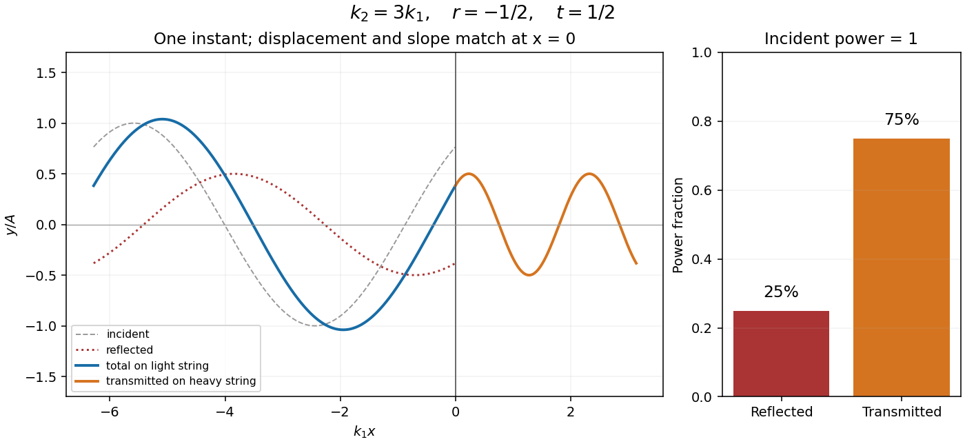
At the same tension, , so , and . The transmitted power fraction is not , because the two strings have different wave impedances. Using the energy flux of a transverse string wave,The reflected fraction is , so . The transmitted displacement amplitude is and its wavelength is . The negative indicates a reflected phase reversal; it does not mean negative reflected energy.
The three nearly horizontal segments have lengths . To first order in small transverse slopes, the upward force on the first point mass is . The force on the second is . Applying Newton's second law to masses therefore givesThe approximation treats the string as massless, retains the imposed equilibrium tension and neglects gravity, as stipulated.
Let and seek a normal mode . Its eigenvalue equation isor , where . ThusThese are angular frequencies; the corresponding ordinary frequencies are .
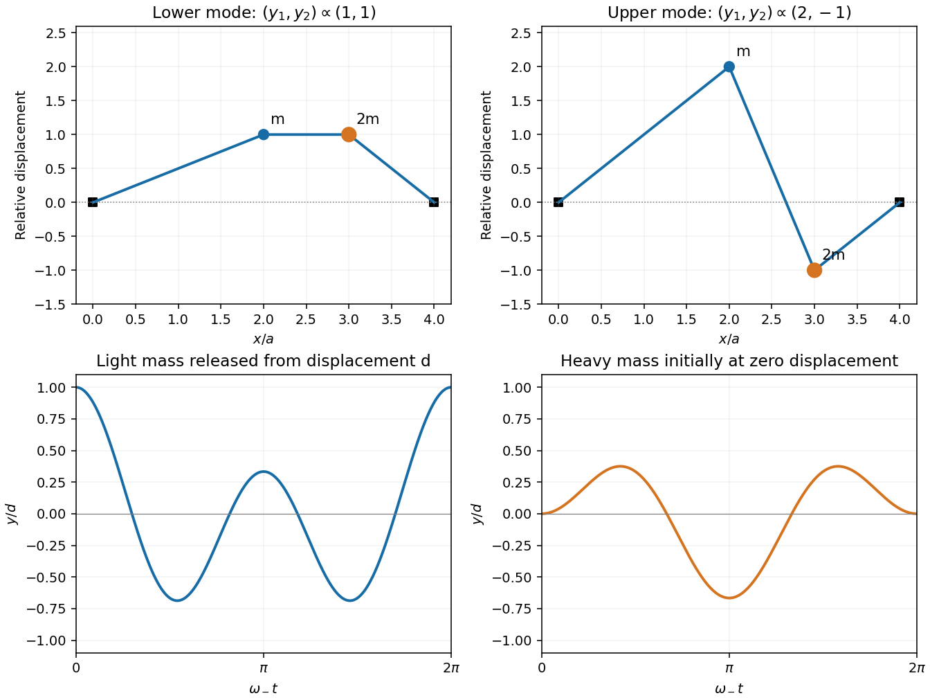
For , the first eigenvector equation gives . For , it gives . ThereforeThe lower mode moves the masses in phase with equal displacements. In the higher mode they move in opposite directions, with the lighter mass's amplitude twice that of the heavier mass. Their eigenvectors satisfy mass-weighted orthogonality with respect to the physical mass matrix , although their ordinary Euclidean dot product is nonzero.


The independent normal modes span the two displacement coordinates. With arbitrary real constants , the general real solution isFour constants are required for two second-order ordinary differential equations, corresponding to two initial displacements and two initial velocities.
Release from rest gives . At , and , so . ConsequentlyThe frequency ratio is exactly two, so both motions repeat after . These are commensurate normal modes, rather than a pair of nearly equal frequencies producing slow beats.
For with continuous second partial derivatives near , its multivariable Taylor expansion iswhere all displayed derivatives are evaluated at . Continuity of the second derivatives justifies equality of the mixed partials and the stated remainder. A cubic-order remainder requires additional regularity.
The notation means the derivative with respect to while is held fixed:For a differentiable function, its first-order height change is . If both coefficients vanish, the tangent plane is horizontal and every directional derivative vanishes: the surface is flat to first order at that point. It need not be constant in a neighbourhood; at the origin is a counterexample. Existence of coordinate partials alone, without differentiability, would not justify this tangent-plane conclusion.
At a stationary point, the linear terms vanish, so , with , , . Let be the Hessian determinant. For , completing the square givesThe second-derivative test therefore yieldsWhen the quadratic form is indefinite, including the case , . When , the quadratic approximation is degenerate and the test is inconclusive: higher-order terms may produce a minimum, maximum or saddle. For nondegenerate cases the quadratic term dominates the Taylor remainder sufficiently close to the point.
The gradient components are and . Their real simultaneous zeros are and . The Hessian matrix is diagonal:At the origin it is positive definite; at each other critical point it is and indefinite. HenceThere are no local maxima. The contours are symmetric under either coordinate reflection. Small positive levels have a closed component surrounding the minimum; these meet the saddle-level separatrices at level . That critical contour has the useful exact form . Other components extend toward large , where the term makes the function unbounded below.
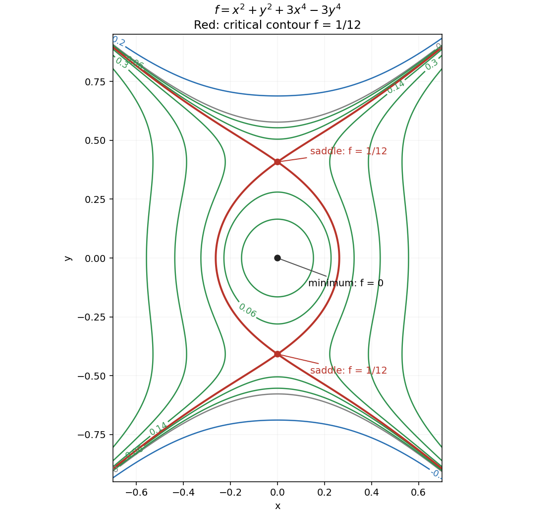
Contours near a minimum and two saddle points, including the critical level one twelfth
. Details. 
Articles by others on the same topic
There are currently no matching articles.