The two free indices are the row and column indices of a matrix. The Kronecker delta has value one on its diagonal and zero off it, so the answer is the identity matrix .
This is the incorrectly formed expression. In the Einstein summation convention, an index in a term is either free and occurs once, or summed and occurs twice. Here occurs three times in the same product, so it cannot consistently be classified as either. Renaming a dummy index before multiplying would give a valid different expression, such as , but does not make the printed expression valid.
The contracted Kronecker delta is . The other scalar contraction is , while is the th component of the matrix transpose applied to . Hence the resulting vector isBoth terms have the same single free index , as required by the Einstein summation convention.
Compare with . The scalar factors commute, so the answer isThe order of the contracted indices matters because the Levi-Civita symbol is antisymmetric.
Interchange the two dummy indices . The product is symmetric under this interchange, while the Levi-Civita symbol changes sign. Thus the contraction equals its negative and is the zero vector, equivalently .
For the unheaded continuation, write the vector triple product asThe Levi-Civita symbol contraction is . One way to check its sign is to fix distinct : the only nonzero term has the remaining index, and the pairs contribute respectively. When , both sides vanish. Contracting with the vectors now gives both requested notations:If and are orthogonal, then . With the specified , the perpendicularity of the cross product gives . ThereforeThe same answer covers the degenerate case in which one of these two vectors is zero.
Expanding the cross product component by component gives its cross-product matrix:It is a real skew-symmetric matrix and annihilates . By the vector triple product,so for a unit vector . Choose a unit vector and put . Then is an orthonormal basis and , , . Thus the characteristic polynomial is and the cross-product matrix spectrum isOver the complex numbers, corresponding eigenvectors are , , and . Only the zero eigenvalue has real eigenvectors.
For the specified third coordinate axis, direct multiplication givesIts zero eigenspace is , and its eigenspace is the whole plane . Hence the eigenvalues of are , with every nonzero vector in the appropriate eigenspace an eigenvector.
A real number is the supremum of a nonempty set if every satisfies and no smaller real number is an upper bound. Equivalently, for every there is with . A greatest element, or maximum, additionally belongs to .
Let and suppose . Fix . The approximation property gives at least one element of in . If there were only finitely many, they would have a largest value . Every other element of is at most , so would be an upper bound for the whole set. This contradicts the definition of the supremum. Therefore there are infinitely many such elements, the accumulation below an unattained supremum.
For a counterexample when the supremum is attained, take . Its supremum and greatest element are both zero, while every interval contains no elements of .
Suppose, towards a contradiction, that for every , where . Choose a radius strictly between and , and take any with . ThenThe geometric series on the right converges because its ratio lies in . The comparison test for series therefore gives absolute convergence of the power series at , contrary to the defining property of its radius of convergence. Thus is unbounded in whenever . This is the bounded power-series terms force interior absolute convergence principle. The case has no points outside its convergence disk and the assertion is vacuous there.
Every possible radius of convergence is realized by an explicit power series:For the first, consecutive absolute terms have ratio , so at every they eventually grow and do not tend to zero; at zero the series is defined. The middle geometric series converges absolutely exactly for , and outside that disk its terms grow. The last has consecutive-term ratio , so the ratio test gives absolute convergence for every finite . These arguments use the necessary zero-term condition for convergence, the comparison test for series, and absolute convergence of a geometric series with ratio less than one; they do not assume convergence on the boundary.
The complex exponential function factorizes as . HenceThe real exponential multiplies both components; it does not change the argument.
Using and collecting real and imaginary terms gives the complex cosine identity . ThusThe sign follows from the factors and in the two complex exponentials.
For , write with . The complex logarithm has values , . ThereforeFor a specified single-valued branch, choose the corresponding continuous determination of the argument. In particular, the principal value uses ; it is not represented correctly by in every quadrant. The complex logarithm is undefined at zero.
For , rationalizing the denominators gives and . Their imaginary parts cancel, soThis also follows because the summands are complex conjugates.
The cubic terms are the expansion of . Subtracting therefore givesHere the expression is a polynomial in and its complex conjugate, rather than a holomorphic polynomial in alone.
For the unheaded continuation, set in the food equation. The two square roots are , so exponentiating givesBoth values have and hence lie strictly inside the disk. Both also have the indicated principal logarithms. Allowing the multivalued complex logarithm produces no additional points: the only permitted values of are still the two square roots already used.
For drink, the PDF squares only the denominator. Put . Its numerator is and its unsquared denominator is , which is nonzero unless . Multiplying the equation by this denominator squared and equating the real part and imaginary part yieldsthat is and . If , the real equation gives or , and zero is excluded. If , then , but the real equation would require , impossible for real . ThusIt lies on the allowed disk boundary, and direct substitution gives . The denominator-only square matters: squaring the entire quotient would define a different locus.
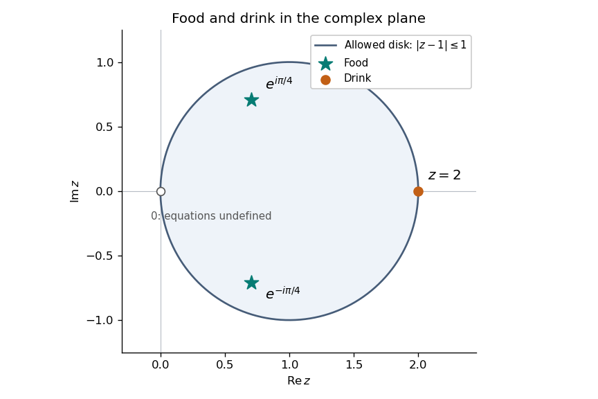
Food points inside the allowed complex disk and the unique drink point on its boundary
. Details. 
The matrix rank is the dimension of its column space, equivalently the dimension of the image of the corresponding linear map. The equation is solvable precisely when , equivalently when the augmented matrix has the same rank as . If is one solution, every solution is with , since subtracting any two solutions gives a kernel element. The rank-nullity theorem gives .
Consequently, for rank three there is one solution for every , namely . For rank two there are no solutions outside the column plane, and an affine solution space of a linear equation of dimension one when consistent. For rank one, consistency requires to lie on the column line and the solution set is an affine plane of dimension two. For rank zero, : the solution set is all of if , and empty otherwise. These descriptions include homogeneous systems, whose solution spaces pass through the origin.
The sphere has normal at the specified point, so its tangent plane isA general straight line through the origin is , , for a fixed nonzero direction . To express the intersection using a matrix, choose independent vectors spanning . The line is exactly the intersection of and , henceThe first two rows have rank two. The third is independent of them exactly when . In that case the rank is three and the unique intersection isGeometrically the line crosses the tangent plane transversely. If , the matrix rank is two: its third row is a linear combination of the first two, but the corresponding right-hand-side combination would be zero rather than two. The system is inconsistent and there is no intersection. The line is parallel to the tangent plane and cannot lie in it, since it contains the origin while the plane does not. Thus no choice of a genuine direction produces an infinite intersection in this particular problem.
For , define the orthogonal projection of onto its span byThe first is parallel or antiparallel to , or zero, and . This proves the decomposition. If as well, comparison with yieldsIndeed shows that the ratio lies in . There is a unique with this cosine. The definition is symmetric in the two vectors, unchanged by orthogonal coordinate changes and positive rescaling, and agrees with ordinary plane geometry in their span: projecting a unit vector onto the other gives its cosine. Parallel, perpendicular and antiparallel directions give respectively. The zero vector has no defined angle; if , the nonzero-axis projection formula itself must not be used.
The vertices of the centered hypercube are sign vectors . A body diagonal identifies and , hence there are such diagonals. If two sign vectors disagree in positions, their dot product is . For odd this integer is odd and cannot be zero. Thus no two body diagonals are perpendicular in odd dimension, by the orthogonality of hypercube body diagonals.
In four dimensions, mutually orthogonal nonzero vectors are linearly independent, so at most four mutually perpendicular diagonals are possible. Four are achieved by the directionsEach has squared norm four and every distinct pair has zero dot product; these are the rows of a Hadamard matrix. Therefore the maximum is four.
For distinct diagonals, the Hamming distance is ; would represent the same line. Oriented vertex directions therefore give cosines . The angles areFor unoriented diagonals, the usual smaller angle between the lines is or ; the supplementary intersection angle also occurs when the two rays are chosen oppositely. Stating this convention avoids counting a line and its reverse as different diagonals.
Use matrix notation and set , , . Contracting the proposed decomposition with and taking its trace, using the stipulated transverse and trace conditions, givesThese relations determine both scalars and the transverse vector uniquely:The last expression obeys directly.
To construct and check the remaining symmetric matrix, use the orthogonal projection matrix onto , and defineBoth terms are symmetric, , andExpand with . The mixed terms are and , while and . Consequentlyand the displayed coefficient equals . This proves existence as well as the axis decomposition of a symmetric matrix formulas.
For the dimension count, choose an orthonormal basis whose third axis is parallel to . The vector has two transverse components. The conditions and symmetry set the third row and column of to zero, leaving a symmetric block. Its zero trace leaves two independent entries, of the form . Together with the two independent scalars , the total is parameters, exactly , the dimension of real symmetric matrices. The recovery formulas also prove uniqueness, so this is an actual parameterization without redundant degrees of freedom.
For , . The upper bound has telescoping partial sums, bounded by one. The positive partial sums of the original series are consequently bounded by two and increasing, so they converge as a monotone bounded sequence. The series converges absolutely. This also supplies the case of a p-series without requiring its exact sum.
For odd , the denominator is ; for even , it is . There is no zero denominator in the printed index range. For all ,The comparison test for series with the convergent p-series gives absolute convergence. In fact the consecutive pair contributes , so the sum is the same as . Positivity justifies this paired reordering; an alternating-sign appearance in the denominator does not make this an alternating series.
Let denote the summand. Its denominator is positive for every : odd gives , while even gives . Dividing numerator and denominator by their highest powers givesThe terms are positive for sufficiently large , so the limit comparison test with the divergent harmonic series gives divergence to . More explicitly, for the numerator is at least and the denominator is at most , giving . Any finitely many early negative terms change partial sums by only a finite constant and cannot prevent divergence of this positive tail.
The PDF has the doubly exponential denominator . For its positive summands, the successive-term ratio isThus the ratio test proves absolute convergence. Concretely, the tail is eventually dominated by a geometric series of ratio ; the polynomial numerator cannot offset the doubly exponential decay.
For a bounded real function on , take a partition . Its lower and upper Darboux sums areThe function is Riemann integrable when ; the common value is its Riemann integral. Equivalently, for every there is a partition with . A continuous function is bounded and Riemann integrable on each compact interval, so all the following integrals exist.
Set for . Strict decrease gives for . Integrating, with strict inequalities because the difference is positive on interior subintervals, givesThe intermediate value theorem produces with , and strict monotonicity makes this point unique. Thus there is exactly one such in .
For the given exponential function, , soThe preceding strict bounds already prove ; no limiting value at zero needs to be included in its domain.
For differentiability, a continuous strictly monotone function has a continuous inverse on its range. If it is differentiable at an interior point with , the inverse is differentiable at , with derivative . Indeed, setting , inverse continuity gives as , andThis one-dimensional inverse result needs no assumption that is continuous. It is enough here that is differentiable and at every positive argument.
The fundamental theorem of calculus and the quotient rule giveNow and , so the inverse derivative formula applies at every relevant point. The monotone mean-value point of an integral average satisfiesBoth numerator and denominator are negative. For the exponential example, this also agrees with , since for .
To prove the required zero-existence statement directly, let and . This set is nonempty and bounded. Continuity and the strict signs at the endpoints give a right neighbourhood of with negative values and a left neighbourhood of with positive values; consequently . If , continuity would give points of to the right of , contradicting its upper-bound property. If , continuity would give an interval immediately to the left of containing no points of , contradicting the approximation property of its supremum. Hence for some , proving this form of the intermediate value theorem.
For the half-interval claim, put on . It is a continuous function andIf either endpoint value is zero, it supplies the answer. Otherwise the signs are opposite, so the intermediate value theorem, applied also to if necessary, gives an interior zero. Thus for some .
For general positive integer , define on . At its grid points,If a sampled value is zero, it is the desired point. If none is zero, not all sampled values can have the same sign, so two have opposite signs; continuity gives a zero between their grid points. This proves the horizontal chord of reciprocal-integer length:For the interval is the single point zero, which works by the endpoint equality itself. The proof does not require a differentiable function or a periodic extension.
If is constant, any interior point works. Otherwise the extreme value theorem gives an attained maximum and minimum on the interval, and at least one of them differs from the common endpoint value. That extremum must occur at an interior point . At an interior maximum, for small positive the difference quotient is nonpositive, while for negative it is nonnegative. Existence of the common derivative forces it to be both nonpositive and nonnegative, hence zero. The same argument with inequalities reversed applies to an interior minimum. This proves Rolle theorem, including the derivative-at-an-extremum step rather than assuming it.
Now let the nonconstant polynomial have distinct real roots , with multiplicities adding to its degree . If and , differentiation givesThe bracket is nonzero at , so its multiplicity as a root of is exactly . These roots already contribute real roots counted with multiplicity. Rolle theorem supplies an additional root of in each of the disjoint intervals . These additional roots are distinct from each other and from all the .
We have therefore exhibited at least real roots counted with multiplicity. The derivative has degree , so there is no room for any additional nonreal roots. Every root of is real. This is the Rolle root count with multiplicities; for the nonzero constant derivative has no roots, as expected.
For failure of the converse, takeThe derivative has only the real root zero, of multiplicity two. But and the quadratic factor has roots , which are nonreal. Thus real-rootedness of the derivative does not imply real-rootedness of the original polynomial.
Articles by others on the same topic
There are currently no matching articles.