Lagrange theorem for polynomial congruences says that a nonzero polynomial of degree over a field has at most distinct roots of a polynomial. It follows by repeatedly factoring out at a root. Over the finite field , the only solutions of are and : these are distinct because is odd, and the root bound excludes any others.
Every nonzero element has a unique multiplicative inverse. Pair each element of with its inverse. All pairs of distinct elements contribute to the product; the only unpaired elements are and . Thus Wilson theorem follows:If Lagrange's theorem is formulated for finite groups, it states that the order of a subgroup divides the order of the group; in particular every element of has order dividing . The inverse-pairing proof above establishes the required congruence directly.
Put and let . The even residues are precisely the negatives, in reverse order, of the odd residues . Hence their product is in the finite field . Applying Wilson theorem givesThe initial factor can be omitted, soFor the product is empty and equals , consistently with the formula.
Let . Choose a unit complex number normal to a supporting side of this convex set, withSuch a choice exists explicitly: take , where are the signs of the real and imaginary parts of ; then and the strict inequality is exactly the hypothesis. Set . Since on ,For sufficiently large , the former is strictly smaller than the latter uniformly on . Consequently .
The geometric series now supplies actual approximating polynomials:Choose so the right-hand side is below . This proves the required uniform approximation without assuming a general approximation theorem.
Yes. Take exterior poles . By part (i), choose a polynomial withFor any fixed , , and therefore . The triangle inequality provesThis is pointwise convergence. It is not uniform convergence on : every polynomial is bounded on the closed diamond, whereas is unbounded as along .
A Kleinian group is a discrete subgroup of , acting by Möbius transformations on the Riemann sphere, equivalently by orientation-preserving isometries of hyperbolic space .
Consider the classes ofThey generate a discrete subgroup because their matrix representatives have integer entries: a sequence of such matrices converging to or is eventually constant. On the real projective line set and . For every nonzero integer ,The last inclusion follows from when ; also . The ping-pong lemma therefore says that the subgroup is the free product . Both generators have infinite order, soa free group on two generators. The ping-pong inclusions ensure that no nonempty reduced word can act as the identity, which is the essential freeness argument.
For a binary linear code , its rank is its dimension of a vector space . Use the weight enumerator conventionwhere is the Hamming weight. This convention is essential here: counts words of weight , rather than zero words. There are codewords, so .
There is only one binary word of weight , namely . Thus precisely when . If this holds, the linear map is a bijection of and replaces weight by ; hence . Conversely this symmetry gives , because the zero word is the unique word of weight zero.
The repetition code consists of , givingThe single parity-check code consists of all words of even weight. Exactly words have weight , so the binomial theorem gives
A generalized linear model has independent responses whose distributions belong to an exponential family:Here the expected value and variance are and . A specified one-to-one link function connects the mean to the linear predictor: . The canonical link function is .
In binomial regression, independently, with known trial counts and probabilities related to the predictor. The logistic regression and probit regression specifications are respectivelyHere is the standard normal distribution function. The binomial log-density contains , so its natural parameter is the log-odds: the logistic link is canonical. If the response mean is written as , the canonical link is .
The physical state space is the positively invariant set , : adding the equations gives zero, and the vector field points inward at each coordinate boundary. At an equilibrium point, either , giving , or . ThereforeA positive endemic equilibrium exists exactly when .
For , put . Since ,The last limit follows either by evaluating the exponential integral (with a term when ), or by splitting it into an early decaying part and a late part with uniformly small . Hence for every physical initial condition. Although immune numbers need not decrease monotonically initially, both infected and immune numbers tend to zero.
At the endemic equilibrium, the Jacobian matrix of the subsystem isA disturbance proportional to therefore obeysBoth coefficients are positive. Real roots have negative sum and positive product; complex conjugate roots have real part . Thus the endemic equilibrium is asymptotically stable by linear stability analysis.
For the iteration of a map , a fixed point satisfies . If , the bracket is strictly positive, so the sole fixed point is . Its multiplier of a periodic orbit of an iteration is , whose modulus is below one. Thus by fixed point stability for an iteration.
For , the multiplier at the origin exceeds one, so it is unstable. The other fixed points areUsing fixed point stability for an iteration, exactly when , and when . HenceThe endpoint has multiplier and requires nonlinear analysis, which is not part of the asserted open intervals.
On the map is positive. Its maximum occurs at and equals . Thus if , then . Since is odd, also . Induction givesThe case is constant. These intervals are positively invariant sets for the discrete dynamical system.
Put . On , the extrema of occur at or the endpoints. The corresponding values are , including the endpoint value . ConsequentlyThus is a trapping region andIt contains a neighbourhood of the origin. Sign changes are possible because has opposite sign to for .
The numbers are the nonzero zeros of a function , repeated according to their multiplicity. The displayed Weierstrass factorization theorem formula uses genus-one Weierstrass elementary factors and a linear exponential factor; it applies under the corresponding growth assumptions, rather than to every arbitrary entire function.
Apply it to the entire function , with its removable value . Its zeros are , each simple, and because is even. Pairing the factors at and givessoThe product converges uniformly on compact subsets because . Away from the integers its logarithmic derivative can be taken term by term: the resulting series also converges locally uniformly, its terms being . HenceThis is an identity of meromorphic functions, understood away from their poles.
Noether theorem associates a conserved quantity to a continuous symmetry of the Lagrangian (with the usual boundary-term correction if the Lagrangian changes by a total derivative). The angles and are cyclic coordinates, so for the heavy symmetric topTime-translation symmetry gives conserved energy, whose Hamiltonian expression isIt is quadratic in the momenta; . Eliminating the cyclic velocities and putting , so , yieldsThe first term has degree three and the second degree two, displaying the cubic governing nutation.
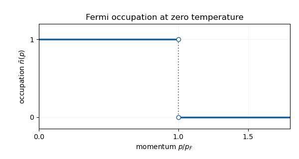
As , the Fermi-Dirac distribution tends to a step function: for , and for . The value at equality is immaterial to the integrals. The Fermi momentum is defined by : the Pauli exclusion principle fills the lowest available states and forbids multiple occupation of a state with a fixed spin. Thus the sketch is a horizontal line at one up to , followed by a jump to zero.
In the ultrarelativistic, , givingEliminate to obtainThe supplied expression for includes rest energy; in this limit its leading term is also the leading kinetic energy.

Electrical neutrality gives at the accuracy of the proposed estimate. With and , the degenerate electron gas result givesThe gravitational potential energy is . Both scale as , so in the strictly ultrarelativistic approximationFor sufficiently large mass the bracket is negative, and contraction lowers the energy without bound in this model: electron degeneracy pressure cannot halt collapse. Equating the scales gives the Chandrasekhar massBelow this scale, the strictly ultrarelativistic expression alone has no finite-radius energy minimum; including the transition to nonrelativistic electrons produces the stable white dwarf branch. Composition and the stellar density profile supply the numerical factors omitted by this scaling estimate.
For , the Dirichlet series is absolutely convergent. A finite product over primes can be expanded into absolutely convergent geometric series. By unique prime factorization,The omitted integers are all greater than , so the difference from has modulus at most . ThusThis defines the infinite Euler product as the limit of finite products. Its absolute convergence also follows from , with for sufficiently large .
Since , the assumed identity becomesfor , where is the fractional part. ConsequentlyTo justify the analytic continuation, on any compact subset of this half-plane choose with . The integrand is bounded by , an integrable function. Each derivative with respect to is bounded by a constant times , also integrable. Differentiation under the integral is valid, so the right-hand side is holomorphic throughout the half-plane, including .
Let . If , minimality is immediate. Otherwise suppose a polynomial of degree at most has strictly smaller error. At each alternation point,Thus changes sign between every pair of consecutive . By the intermediate value theorem it has at least distinct roots of a polynomial, contradicting its degree bound. ThereforeThis is the sufficiency direction of the Chebyshev alternation theorem.
Fix distinct nodes . The Lagrange interpolation formula expressesThe vector of node values is bounded in , so the Bolzano-Weierstrass theorem supplies a subsequence converging to . Put , of degree at most . Because the are fixed bounded functions,along that subsequence. The reverse triangle inequality implies . Thus a best uniform approximation exists, with no appeal to an unproved abstract existence result.
Enumerate the finite set increasingly, , so alternating signs refer to spatial order. This is the enumeration needed for the interpolation construction below. The Lagrange cardinal polynomials satisfy and have degree .
If the printed indexing were interpreted as an arbitrary fixed permutation, the assertion in (a) would need this qualification. For example with , gives of degree two; for every works. Ordering the nodes resolves the issue and yields the requested minimizer for every set .
The coefficient of in isWith the increasing enumeration, its sign is . Therefore all terms have the same sign , and . The leading coefficient of is . Canceling the coefficient of gives the unique valueBoth interpolants have degree at most , so this single cancellation is equivalent to .
Set using part (a). At every node,If , the error vanishes. Otherwise any degree-at-most- polynomial with strictly smaller error would make have alternating nonzero signs at the increasingly ordered nodes (reversed globally if ). It would then have at least distinct roots by the intermediate value theorem, impossible. Hence
The reaction–diffusion system for amoebae contains local reproduction and density-dependent loss , giving carrying density . The term describes diffusion with coefficient one. The chemotaxis flux is , so its contribution to the conservation equation is . Attraction towards greater chemical concentration requires at the relevant positive densities; negative values would mean repulsion, and zero removes the chemotactic response.
In the chemical equation, is secretion proportional to amoeba density, is first-order chemical degradation, and is chemical diffusion. The cell reaction term permits births and deaths, so the total number of amoebae is not conserved.
For a spatially homogeneous positive steady state, and , givingWrite , , and define . Homogeneous linearization givesThe eigenvalues are , both negative. Hence this steady state is stable to homogeneous disturbances, including the repeated-eigenvalue case, where a possible factor still decays.
The background has , so the linear chemotaxis term is ; derivatives of multiply products of disturbances and do not enter at first order. For a normal mode with and time dependence , put . Thenand the characteristic polynomial isIts linear coefficient is positive for every . Thus instability occurs exactly when its constant term is negative: the roots are then real with opposite signs. The positive quadratic is negative somewhere on precisely whenThereforeAt equality the neutral wavenumber is and . Above threshold the unstable band is , where
Only the Laplacian eigenfunctions whose eigenvalues lie in the intersection of the unstable band with the allowed spectrum can grow. A lower bound removes all unstable modes if , even when the unrestricted threshold in (iii) is exceeded.
If all real wavenumbers above the cutoff are possible, an equivalent strict threshold isIt is unchanged when , and becomes when . A bounded geometry generally gives a discrete spectrum, so the stronger requirement is that an actual allowed eigenvalue falls in the band.
A steady-state bifurcation is a change in the local equilibrium branches or their stability as a parameter varies. At such a bifurcation the Jacobian matrix at the equilibrium has a zero eigenvalue, so the implicit function argument for a unique persistent local equilibrium fails.
For this system,At its eigenvalues are ; at they are . Both have one simple zero eigenvalue at , with the other eigenvalue negative. Interior equilibrium branches, obtained below, meet these boundary equilibria there, establishing the actual bifurcations rather than merely a necessary eigenvalue test.
Near put , , , with . The extended system isThe extended centre manifold for a parameter has , , . Its centre-manifold invariance equation is . The left side starts at degree three. At degree two the right side is , so , with no or term. Substitution givesThe leading normal form of a dynamical system has branches and , exchanging stability at : this is a transcritical bifurcation. In the physical quadrant the interior branch is present only for .
The equations extended across are equivariant under , so near the reduced equation is odd in . To verify its nondegenerate pitchfork bifurcation, set and . ThenThe local centre manifold has , obtained by balancing the quadratic terms of its invariance equation. Consequently : the cubic coefficient is nonzero. This is a subcritical pitchfork, with the two symmetry-related interior branches existing for in the extended plane; only the branch belongs to the physical quadrant.
At an interior equilibrium point, , soFor both values satisfy , giving two physical equilibria. At such an equilibrium,The branch is asymptotically stable by the trace-determinant stability criterion; is a saddle equilibrium. In fact is symmetric, so the stable branch has two negative real eigenvalues.
At the equilibria merge at . Writing , the equilibrium condition is , the characteristic branch geometry of a saddle-node bifurcation. The stable node and saddle annihilate as increases through .
The bifurcation diagram has boundary branches at and at . The former is stable for and a saddle for ; the latter is a saddle for and stable for . The origin is an unstable equilibrium for every ; its branch coincides in this projection with the branch, so it is shown separately in the caption.
The stable interior branch rises from at to at . The unstable interior branch falls from to over the same interval. These meet at the saddle-node bifurcation; at they meet the transcritical and pitchfork points respectively. There is bistability between the lower interior node and for .
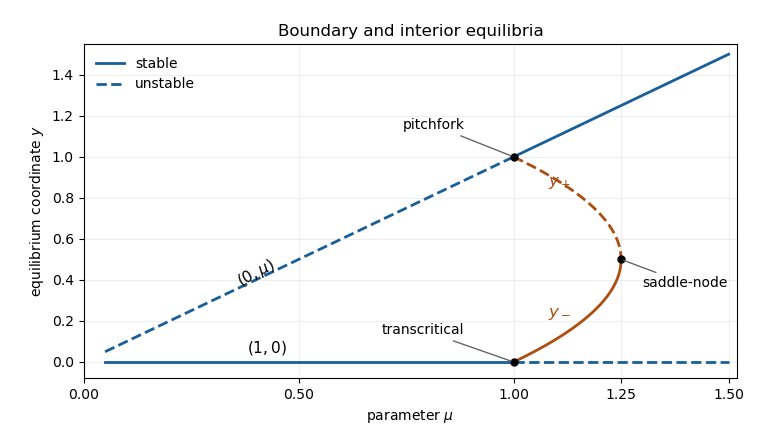
Equilibrium branches and stability for Question 14; the always unstable origin also projects to y equals zero
. Details. 
A fixed comoving volume labels a fixed collection of cold dark matter particles. Their background mass is , which is constant by mass conservation. At the perturbed positions it is . The Jacobian determinant of the Zeldovich approximation map isTaking its reciprocal and using mass conservation givesFor the perturbed field the Poisson equation must be . The displayed background-only right-hand side in the PDF would give no clumping force; it is the background equation, not the full perturbed equation.
Write , where . To linear order,For the longitudinal, curl-free displacement used in the growing Zel'dovich mode, this integrates to , after removing external homogeneous harmonic fields. More generally the force involves only the longitudinal part , which has the same divergence as .
Differentiate twice at fixed and substitute . The terms proportional to cancel using , leavingFor a longitudinal displacement the right side is . Taking minus the comoving divergence gives the general scalar density contrast equation
Both background components are pressure-free, so their densities scale as and is constant. Since and , a power law satisfiesThusFor the plus sign gives a growing mode and the minus sign a decaying mode. At the growing exponent becomes zero, since no gravitating clumping component remains.
When , , so . The redshift relation gives . Even an entirely growing initial mode therefore givesThe perturbation remains far below order unity, so it cannot produce the observed nonlinear gravitational clumping within the stated model. A decaying admixture does not provide the missing sustained growth.
The compactness theorem states that a set of first-order sentences has a model if every finite subset has a model. The Upward Lowenheim-Skolem theorem says that an infinite structure in a language has an elementary extension of every prescribed infinite cardinality .
Add constants for all and the elementary diagram of a structure of : every sentence with these constants true in . Add further constants and sentences for . Any finite subset is satisfiable in , by choosing the finitely many new constants distinctly, since is infinite. Compactness gives a model containing an elementary copy of and at least elements.
For the exact cardinality, start with that copy and all the , a set of cardinality . For every existential formula with parameters from this set that holds in the large model, choose one witness. Also close under the language's functions. Repeat countably many times. At each stage there are at most formulas and finite parameter tuples, so the union still has cardinality . Every existential formula true in the large model with parameters in the union has a witness in the union; an induction on formulas proves that this substructure is elementary. This establishes the exact-size statement without assuming an unproved downward theorem.
A dense total order with is not a well-order: the nonempty set has no least element, since density supplies a point strictly between and any proposed least element.
In the strict-order language, the required axioms areThese axiomatize dense total orders, allowing endpoints. If more than one point is required, add . For a non-strict poset language replace by .
This class is not first-order axiomatisable. If a theory axiomatized the countable dense total orders, it would have as an infinite model. By the Upward Lowenheim-Skolem theorem it would also have an uncountable model, contradicting the proposed restriction. The same argument applies whether countable means exactly countably infinite or at most countable.
This class is also not first-order axiomatisable. Suppose such a theory had an uncountable dense-order model . Its language is finite. Starting with a countably infinite set of elements and repeatedly adjoining witnesses for all existential formulas with parameters already chosen yields a countable elementary substructure: there are only countably many formulas and parameter tuples at every stage. The induction-on-formulas argument from part (i) proves elementarity. The substructure satisfies every sentence of the theory, yet is countable, a contradiction. This is the witness construction underlying the Downward Lowenheim-Skolem theorem.
Well-orders are not first-order axiomatisable. Suppose a theory axiomatized them. Enlarge the language by constants and addEvery finite subset of the resulting theory has a model in the well-order : assign its finitely many constrained constants to a sufficiently long finite descending chain. Thus the compactness theorem supplies a model of with an infinite descending chain. The set of the has no least element, contradicting well-ordering. This shows why the second-order assertion that every nonempty subset has a least member cannot be replaced by a first-order theory in the poset language.
The Turán graph is the complete -partite graph whose vertex-class sizes differ by at most one; empty classes are allowed when . Its edge count is . Turan theorem states that every -vertex graph containing no has at most edges.
Here is a symmetrization proof, including the equality case. Let be any -free graph maximizing the edge count. If nonadjacent have unequal degrees, replace the lower-degree vertex by a twin of the higher-degree vertex: this increases edges and cannot create a forbidden clique, since any new clique containing the twin corresponds to an old clique containing its model. Thus all nonadjacent pairs have equal degrees.
If such had distinct neighbourhoods, choose (their equal degrees ensure such a vertex exists), and clone onto . The new graph has the same maximum number of edges and is still clique-free. Originally and were nonadjacent, so . After cloning, loses precisely its edge to , while keeps its degree. They remain nonadjacent but now have different degrees, contradicting the preceding necessary property of every extremal graph. Hence nonadjacent vertices have identical neighbourhoods.
Nonadjacency together with equality is therefore an equivalence relation, making complete multipartite. It has at most classes, otherwise choosing one vertex from each of classes gives a clique. For fixed total size, is minimized by classes balanced as equally as possible: splitting a nontrivial class when fewer than classes are used adds edges, and moving a vertex from a class of size at least two greater than another also adds edges. Thus every extremal graph is , up to isomorphism. This proves both the bound and its equality characterization. In particularFor the bipartite assertion, take a maximum matching in a graph of edges. No edge joins two unmatched vertices. Let be its endpoints. For each matched pair , both and cannot have neighbours outside : those two neighbours lie in opposite vertex classes and would replace by two disjoint edges, increasing the matching. Thus at most edges from this pair lead outside , giving . There are at most edges within . ConsequentlyIf , necessarily .
Finally let be the three classes of the triangle-free graph. If , the desired bound is immediate. Otherwise set . The preceding result gives disjoint edges. For each edge , the -neighbourhoods of its endpoints are disjoint, or there would be a triangle, so . The other vertices of each have at most neighbours in . HenceSince ,Equality is attained by retaining every and edge and no edges.
The cyclotomic Galois group theorem statesfor coprime to , with , where is the Euler totient function.
Choose with . The roots of are , so contains every root. Conversely their ratios generate the roots of unity, so is precisely the splitting field of over . In characteristic zero this polynomial is separable polynomial, since , and a splitting field of a separable polynomial is a Galois extension.
Each automorphism over sends to . The map embeds into the cyclic group : it is multiplicative because the automorphisms fix roots of unity, and injective because generates . Hence this group is cyclic, of order dividing .
For a Galois intermediate field , restriction of automorphisms gives an exact sequenceSurjectivity uses the extension theorem for embeddings into a normal splitting field. Both kernel and quotient are abelian, so the commutator subgroup of lies in the abelian kernel. Its next commutator subgroup is trivial. Thus
For prime, and the cyclic group has order either or . ThereforeThese correspond respectively to being or not being a th power in . In fact it is a th power in precisely when it is a th power in . To see the nontrivial implication, suppose and . Taking the field norm gives with . Then , so is already a rational th power.
Both degrees occur: gives , while is not a rational th power and gives . This includes , with possible degrees and .
For a character of a subgroup , the induced character isIt is the character of the induced representation , and has degree . The character inner product is . Substituting the displayed formula and putting yieldsThus Frobenius reciprocity isNow assume index two, so is normal. Choose and write . Directly from the induction formula,If , this norm is one, so induction is irreducible of degree : is monogamous. If , the norm is two. Since a norm is the sum of squared nonnegative integer multiplicities, induction is the sum of two distinct irreducibles, each once. Each is related to , so its degree is at least by restriction and reciprocity; their degrees sum to , forcing both to have degree . Thus is bigamous.
Every irreducible of restricts to a nonzero sum of irreducibles. Choose a constituent . If is bigamous, is one of its two degree- partners; since its restriction already contains a degree- constituent, . If is monogamous, and , giving precisely two distinct monogamous partners of equal degree.
The complex irreducible character degrees of are , with squared sum . Conjugation by the outside coset preserves degrees, so it fixes the unique degree-, degree- and degree- characters and either fixes or swaps the two degree- characters. The two possibilities for areBoth lists have squared sum . They occur for and respectively; in , odd conjugation swaps the two classes of -cycles and hence the two degree- characters.
A simplicial approximation to is a vertex map satisfying the open-star conditionfor every vertex . Here an open star consists of points whose barycentric coordinate at that vertex is positive. This condition ensures that the images of the vertices of every simplex span a simplex of , and the vertex map extends linearly over simplices.
To triangulate , order the vertices of each complex consistently. For each product , use the simplices whose vertices follow monotone lattice paths from to , taking a step in one coordinate at a time. These prism triangulations agree on faces and cover the product.
If both approximate , choose in the relative interior of a simplex . Then belongs to the open star of every vertex of . Hence belongs to every open star of and . Its unique carrier simplex in contains all these vertices. Thus and are faces of that one simplex, proving that are contiguous simplicial maps.
Articles were limited to the first 100 out of 176 total.
Articles by others on the same topic
There are currently no matching articles.