For an odd prime , the Legendre symbol is if , if is a nonzero square modulo , and otherwise. Euler's criterion statesIf both sides vanish. Otherwise write for a primitive root . The squares are precisely the even powers of , while has order two and therefore equals . Hence , proving the criterion and the useful special case .
For odd , . Every prime divisor of this number is odd, and , so . Euler's criterion forces , hence or . A product of such primes can be only if a prime occurs to an odd power.
Suppose the primes were . Choose the odd integer (or for an empty list). None of these primes divides , since the latter is modulo each . Yet the preceding argument gives a prime divisor , outside the list. This contradiction proves infinitely many primes congruent to modulo .
The closure is closed and bounded in , hence compact by the Heine-Borel theorem. It is nonempty. The extreme value theorem therefore gives a point of the closure at which the continuous function attains its maximum. The closure, rather than the open domain, is essential.
At an interior local maximum, the second derivatives in both coordinate directions are nonpositive: restrict the function to each coordinate line and apply the one-variable second-derivative test. Thus there, contradicting . Since a maximum exists on the closure, a maximum lies on the boundary.
For , use the weak maximum principle for elliptic operators perturbation . Its Laplacian is at least , so the preceding argument puts its maximum on the boundary. If , then, for any ,Letting gives . The boundary is compact, so this maximum is attained. This proves the weak weak maximum principle for elliptic operators even when the Laplacian may vanish.
Apply the weak weak maximum principle for elliptic operators to the harmonic function and to . Their boundary maxima are both zero, giving and on the closure. Consequently .
For a block code, the minimum distance of a code is the minimum Hamming distance between distinct codewords, where Hamming distance counts positions in which two equal-length binary strings differ. We use equal-length codewords, so the fact that the codomain allows arbitrary finite strings creates no ambiguity. Minimum distance means every two distinct codewords differ in at least positions and some pair differs in exactly .
Changing at most bits cannot turn a codeword into another codeword. Testing membership therefore detects every such nonzero error. For , suppose a received word lies within distance of two codewords. The triangle inequality would put their mutual distance at most , a contradiction. Hence the radius- Hamming balls are disjoint and nearest-codeword decoding corrects all errors of weight at most .
For an alphabet of size , start with and the standard unit vectors in . Their minimum distance of a code is one. Repeat every coordinate times; every distance is multiplied by , so the resulting code has minimum distance of a code exactly . A one-letter alphabet has no pair of distinct codewords and therefore no finite minimum distance of a code under this definition; the construction concerns the usual nontrivial coding situation.
The standard normal distribution function givesThe observations are independent Bernoulli random variables, because the original errors are independent. Thus the probit regression has intercept and coefficient vector . With the specified known and , recovery isThe scale would not be recoverable from threshold data alone if were unknown.
Substitution of the separated exponential profile into the age-structured population equation gives . ThereforeFor , the birth boundary condition cancels and becomes the Euler-Lotka equationThe survival probability to age is for constant death rate. Hence the expected lifetime offspring count, or net reproduction rate, isThe Gamma integral evaluates the Euler-Lotka equation as , requiring . Its real solution and profile areThus , and gives positive growth. The profile is a nonzero formal separated solution for all positive ; a finite total population additionally requires , equivalently . A decaying-in-time mode need not have an integrable age profile.
Introduce the Mellin transform integral , valid for . A keyhole contour for with has residues and , with the latter argument . The two sides of the positive-axis cut give . The small and large arcs vanish in this strip; simplifying the residue theorem identity yieldsDifferentiation under the integral is valid on compact substrips because the extra is dominated at both endpoints. ThereforeAt , the requested values are
The principle of stationary action says that the physical path makes the action stationary under smooth variations with fixed endpoints . It need not minimize the action. Differentiating and integrating by parts givesThe fundamental lemma of the calculus of variations then gives the Euler-Lagrange equation
Use , the bead's distance from the pivot, and , the rod angle from downward vertical. The kinetic energy is . If the identical springs have common natural length , their potential is . Its -dependent part is ; the unspecified common natural length changes only an additive constant. Gravity contributes . Consequently the Lagrangian may be taken asThis uses the illustrated symmetric two-spring arrangement without assuming an unstated natural length.
Apply the Euler-Lagrange equation separately to and :The first equation balances radial inertia, centrifugal motion, gravity and the net spring force. The second is the angular-momentum equation . For it is equivalently .
Relative positions and velocities measured from galaxy are and . Spatial homogeneity says that the same position-to-relative-velocity rule applies from every galaxy. Thus . Taking and putting , gives additivity . For a continuous physical velocity field, additivity implies rational homogeneity and, by continuity, real homogeneity. Thereforefor a position-independent matrix . Regularity is necessary to exclude pathological discontinuous additive functions.
Decompose the given matrix as , whereIts symmetric part is isotropic: no cosmological shear, expansion scalar , and linear scale factor proportional to for . Its antisymmetric part is rigid rotation with angular velocityThe vorticity is . Comoving separations obeyThus all distances grow by the same power, volumes grow as , and the pattern rotates about the fixed axis through angle . Homogeneity alone permits this rotation; full cosmological isotropy would not.
For , let be the binary matrix whose columns are all distinct nonzero vectors of . The binary Hamming code is . Its parity-check matrix has rank since its columns include the standard basis. Hence is linear of length and dimension .
No word of weight one or two lies in , since columns are nonzero and distinct; three columns sum to zero, so the minimum distance of a code is exactly three. The syndrome of a single-bit error is its column of , uniquely identifying the erroneous position. The possible syndromes correspond to no error or exactly one of single-bit errors. Alternatively, every radius-one Hamming ball has words andDisjoint balls therefore cover the whole word space. This proves linearity, one-error correction and perfection. For , the parameters are , giving the 16 messages needed below.
Independence of individual bit errors gives . Independent retransmissions have a geometric distribution with success probability , so the expected total number of transmissions, including the successful one, is . At the supplied values, and .
A Hamming code decoder succeeds on a seven-bit block exactly when there are zero or one errors. Its radius-one decoding regions are disjoint, so an error of weight at least two cannot decode back to the original codeword. ThusNumerically , so only about transmissions are expected. Even accounting for seven rather than four bits per letter, expected bits sent are , compared with . The Hamming method is substantially better under the stated error detection and independent retransmission assumptions.
The Poisson regression uses independent counts with mean and logarithmic link function. Writing for concentration, the fitted predictors for strains are respectivelyThe interaction formula includes concentration, strain indicators and their products. The intercept is the baseline log mean at zero toxin; exponentiating it gives about fleas. Strain coefficients compare log means at zero concentration. Interaction coefficients compare concentration slopes with the common strain. A unit concentration increase multiplies the three means by about , and respectively.
For design matrix , the fitted expected Fisher information is , , since a Poisson count has variance equal to its mean. Standard errors are square roots of diagonal entries of . Each reported Wald test divides its coefficient estimate by its standard error and compares with an approximate standard normal distribution under a zero-coefficient null, conditional on the other terms. Concentration has strong evidence of a negative baseline effect. At zero concentration strain 1 is not significant at 5% (), while strain 2 is (). The strain-1 slope differs strongly from the baseline (); the strain-2 slope has no detected difference (). A nonsignificant difference is not proof of equality. The very significant intercept is a test of mean one at zero toxin, with little scientific relevance.
Relabelling factor levels merges strains 0 and 2 into one group and leaves strain 1 separate. Model retains three intercepts but allows only two slopes: strain 1 versus the common slope of strains 0 and 2. Thus it has five parameters, compared with six in . Model merges both intercepts and slopes for strains 0 and 2, retaining only four parameters. The natural nesting is .
For these nested generalized linear models, the difference in Poisson deviance is an asymptotic likelihood-ratio test statistic with degrees of freedom equal to the parameter difference. Comparing with gives on one degree of freedom, far below : the additional strain-2 slope is unnecessary. Comparing with gives on one degree of freedom, far above : merging the strain-0 and strain-2 intercepts is rejected. Comparing with uses on two degrees of freedom and requires a two-degree-of-freedom threshold, about , rather than the supplied .
is the most appropriate of the three models: retain different strain baselines and the special strain-1 slope, but pool the unsupported strain-2 slope difference. Residual degrees of freedom are ; deviances of this magnitude give no obvious evidence of overdispersion from these summaries alone.
Write and move the factor onto by integration by parts. The differential-equation residual isThus the Laplace integral solution is obtained fromup to a nonzero constant and branch choices. The endpoint factor is proportional to , so the given positive real parts ensure its vanishing at and .
For , choose the directed intervals and ; for , choose and . On each interval choose a continuous branch separately. Equivalently their integrands, after an irrelevant constant phase is removed, use on , on , and on . Exponential decay at the infinite endpoint removes the remaining boundary term.
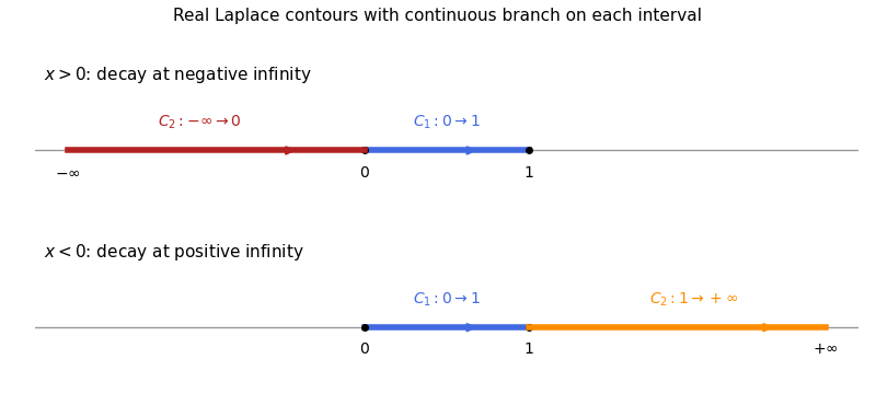
Directed real contours for two Laplace integral solutions: zero to one in both cases, negative infinity to zero for positive x, and one to positive infinity for negative x
. For large positive , has a nonzero leading term proportional to , while is proportional to . For large negative , is proportional to and to . These distinct asymptotics prove independence in each case; the gamma factors are nonzero under the assumptions.
For , integrate on to get . A convenient independent pair on either side of zero isDirect substitution verifies both, and their ratio is not constant. Their singularities cancel in . Since , the solution regular at zero with the required normalization isIts power series supplies the removable value and verifies the equation at the singular point.
Set . Multiplication of the Friedmann equation by givesFor the expanding branch emerging from , . Differentiating where gives , and continuity extends it through a regular turning point. Put . Solving this linear equation with both initial data givesInitially . If , stays positive and strictly increasing; at late times . This universe expands forever.
If , expansion stops when , givingThe physical solution expands from zero and then symmetrically recollapses to zero; negative beyond this interval is not a continuation of a real scale factor.
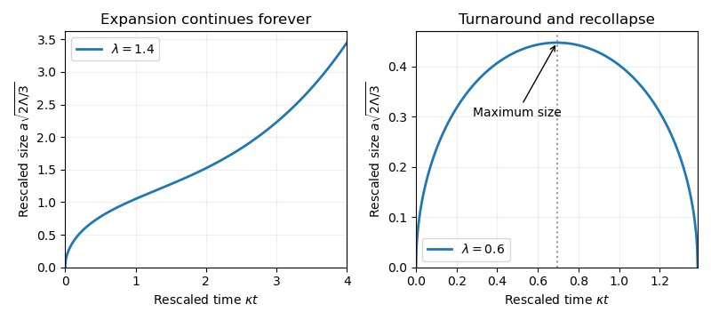
Scale-factor histories for closed radiation universes with positive cosmological constant: eternal expansion for lambda above one and finite-time recollapse for lambda below one
. The completeness theorem for propositional logic states that if and only if . Soundness follows by checking that axioms are tautologies and inference rules preserve truth. For completeness it suffices to prove that every syntactically consistent set has a model.
The deduction theorem for propositional logic used here is: if and only if , in classical propositional logic. A proof is finite, so the union of a chain of consistent sets remains consistent: a contradiction would already occur in one member. By Zorn's lemma, extend a consistent to a maximal consistent set . If , adding yields a contradiction; the deduction theorem gives , and maximal consistency puts in . Conversely and cannot both belong to . Maximal consistency also makes deductively closed.
Assign each primitive proposition the truth value true precisely when it belongs to . The maximal consistent set truth lemma follows by induction on formulas. For negation use the preceding dichotomy. For implication, if or , the classical implication axioms put in ; if and , modus ponens prevents that implication from belonging to . This is exactly its truth table. Other connectives are defined from these or handled by the same induction. The resulting valuation satisfies all of , hence all of .
If , the deduction theorem and classical contradiction rules show is consistent. Its model falsifies , so . This proves completeness.
The propositional compactness theorem says is satisfiable if every finite subset is satisfiable. Otherwise completeness would make inconsistent, and a finite proof of contradiction would involve only finitely many assumptions, contradicting their satisfiability. Equivalently, every semantic consequence of is a consequence of a finite subset. The decidability theorem for propositional logic says there is an algorithm deciding whether a formula is provable with no assumptions: enumerate all truth assignments to its finitely many primitive propositions, check whether it is a tautology, and use soundness and completeness to identify tautologies with theorems. This does not claim an algorithm for arbitrary infinitely presented theories.
Finally, the valuation assigning false to every satisfies all the implications in and falsifies . By soundness, .
A strongly regular graph with parameters is a simple graph in which each vertex has degree , adjacent vertices have exactly common neighbours, and distinct nonadjacent vertices have exactly common neighbours. Its order is often included separately as a fourth parameter.
Let be the adjacency matrix of a graph, the all-ones matrix and the all-ones vector. Counting two-step walks givesBecause , any two nonadjacent vertices have a common neighbour, so the graph is connected. The eigenvalue is simple: for a real eigenvector at , a maximal entry and the averaging equation force its neighbours, and then every vertex, to have the same value. Since is real symmetric, its other eigenvectors lie in , where vanishes. Their eigenvalues are thereforeHere for the present incomplete connected graph. Indeed ; if , then , which conflicts with for an edge. If have multiplicities , dimension and zero trace give and . ThusThese are dimensions of eigenspaces, hence integers. A multiplicity may be zero; that does not affect the conclusion.
Count edges from the neighbours of a fixed vertex to its nonneighbours. Each neighbour contributes such edges, and each nonneighbour receives . With ,The graph is incomplete, so there are nonadjacent vertices and . Substituting into the eigenvalue multiplicity formula gives a multiplicity difference of . This must be an integer. As , is rational and hence an integer; it is positive and odd. Moreover and , so reducing modulo gives . Thus . The value gives , impossible here; the other two give and . Consequently . This is a necessity argument, not a claim that integrality alone constructs either graph.
If the two-dimensional group representation were reducible, Maschke's theorem would split it into a direct sum of two one-dimensional group representations. In a basis respecting that decomposition, every representing matrix would be diagonal. All would therefore commute, contradicting the specified pair. Hence the group representation is irreducible. Complete reducibility over is essential to this argument.
Call the two proposed matrices and . Direct multiplication gives , , and . Both are invertible since . They therefore satisfy every defining relation, and the universal property of a group presentation gives the desired group representation.
Put . The group representations from the preceding construction with , , will be denoted . Their diagonal matrices for have distinct eigenvalues. The only possible invariant lines would be these two eigenspaces, and the matrix for exchanges them. Thus each is irreducible. Equivalently their matrices do not commute, so part (a) applies. The choices and give equivalent group representations by exchanging basis vectors. The displayed range contains exactly one of each pair, and distinct members have different traces at because is strictly decreasing there.
For a one-dimensional character of a representation, write , . The conjugation relation forces , and . Hence there are exactly four choices:For even , for either ; for odd , has and has . Finally,The sum of squares of irreducible representation dimensions proves that these four one-dimensional and two-dimensional group representations exhaust the irreducibles, including where the latter list is empty.
The conjugacy classes are , , for , and two classes containing respectively and , each of size . Conjugation by inverts powers of , while conjugation by changes the exponent of by two; these facts prove the list and sizes. The sizes total .
The complete character table is specified by the following array, with one column for every and one row for every in the indicated ranges:Here ; the four pairs are those in part (ii). In particular, this formula displays both parity cases without concealing the different values when is odd. The zero entries follow because the two-dimensional matrices representing are off-diagonal.
Let be the coefficients of . Each is an algebraic integer. The ring is a finitely generated -module: reduce powers of each generator by its monic integral equation. As is monic, is generated over by , so is a finite -module. It is torsion-free as a subgroup of a characteristic-zero field, hence free of finite rank. Multiplication by on it is represented by an integer matrix. Its monic characteristic polynomial, by Cayley-Hamilton theorem, annihilates . Thus is an algebraic integer. This proves the required transitivity of integrality in this setting.
Every root of the monic is also a root of the monic polynomial , and is therefore an algebraic integer. The coefficients of are elementary symmetric polynomials in these roots, hence algebraic integers because algebraic integers form a ring. They also belong to , so belong to . Consequently .
The cubic has no rational integer root among the divisors of four, so is irreducible. Its polynomial discriminant is . Thus the index is one or two, since its square divides the discriminant.
Set . Using givesand hence . Therefore is integral. The lattice spanned by contains with index two. Changing basis divides the discriminant by four, giving , which is squarefree. An integral lattice of full rank with squarefree discriminant cannot have any further index in the full ring of integers. Henceis the required integral basis. The relations also give , so this ring can equally be generated by .
For with , evaluation , , has in its kernel. It therefore induces a -algebra homomorphism . Conversely, such a homomorphism is determined by , since every class is a polynomial in . Applying it to shows . These constructions are inverse, giving the root-embedding correspondenceIrreducibility ensures the quotient is a field, so each unital homomorphism is injective.
A splitting field of over is an extension generated over by all its roots in which splits into linear factors. A nonconstant irreducible polynomial is separable polynomial when its roots in a splitting field are distinct, equivalently when it is coprime to its formal derivative. For a general polynomial, the convention compatible with the printed assertion is that all its irreducible factors are separable; repeated occurrences of the same factor are allowed under this convention.
For a finite field of characteristic , the finite-field Frobenius automorphism is injective and hence surjective. If an irreducible polynomial had zero derivative, every nonzero exponent would be divisible by . Taking th roots of its coefficients would give , contradicting irreducibility. Thus , and irreducibility gives . Every irreducible factor is therefore separable: finite fields are perfect.
If instead one defines a separable polynomial to mean that the entire polynomial has no repeated roots, the printed claim for every is false: is a counterexample over any finite field. The proof above establishes the precise intended perfect-field assertion; a polynomial has entirely distinct roots if and only if it is also squarefree.
A finite separable field extension of degree has exactly embeddings into an algebraic closure: adjoin finitely many generators successively, and use part (i) to count extensions of each embedding by the distinct roots of the relevant separable minimal polynomial.
For , label these embeddings . For each pair , the equalityexcludes at most one . If the images of agree, the images of cannot agree too, so it excludes none. Since is infinite, choose avoiding the finitely many bad values and put . The images of are distinct, hence its minimal polynomial has degree at least . But gives degree at most . Therefore . Combining generators two at a time proves the primitive element theorem for every finite separable extension over an infinite base field.
A useful closed-cover version of the Seifert-van Kampen theorem is the following. Let with path-connected closed subspaces and basepoint in their intersection. Assume there are open neighbourhoods covering that deformation retract onto , while deformation retracts onto , with the induced inclusions compatible up to based homotopy. ThenThe neighbourhood hypothesis, available for the present finite subcomplex gluing, matters: arbitrary closed covers need not satisfy this theorem.
A Möbius band retracts onto its core circle, with generator ; its boundary represents . The torus has generators and relation . The attaching circle is the circle. Reversing the attaching homeomorphism merely replaces by its inverse and changes no isomorphism type. The closed-cover theorem givesMapping , surjects onto , so the group is infinite. Imposing the extra relation gives the quotient , a nonabelian free product, since alternating reduced words and differ. A quotient of an abelian group would be abelian, so the fundamental group is nonabelian.
Use the convention that the inner product is linear in its first argument. Set and . Orthogonality makes the nearest point in the finite span of the first basis vectors. Since an orthonormal basis has dense linear span, for every a finite linear combination approximates within . For all larger , the nearest-point property gives . Thus the series converges in to even without completeness. Taking inner products with each proves uniqueness of its coefficients.
In the Hilbert-space case, Parseval's identity gives . Completeness makesconvergent. It is linear and preserves inner products and norms, so bounded with norm one. Its inverse is the corresponding map sending to ; equivalently every coefficient sequence of a vector in the basis is also square-summable in the basis. Hence is surjective and unitary. Any bounded map agreeing on the agrees on their dense span and then on all of , proving uniqueness.
Suppose a bounded linear isomorphism with bounded inverse existed. There would be constants such that . Put . Averaging the squared Hilbert norm over all independent sign choices cancels cross terms, giving the generalized parallelogram identityEvery signed sum of the original has -norm . The left side is therefore between and , while the right side is between and . Thus and would be bounded constant multiples of one another for all , impossible unless . Consequently no such normed-space isomorphism exists for .
At a noncritical point a holomorphic map has a local holomorphic inverse. Fibres of a nonconstant map between compact connected Riemann surfaces are finite: zeros are isolated and compactness precludes infinitely many. Around a nonbranch value , choose disjoint inverse neighbourhoods of every point in its fibre. Compactness of the remaining source ensures a sufficiently small disc about has no additional preimages. Its preimage is therefore a disjoint union of open sets each mapped biholomorphically onto that disc. This proves a finite-sheeted unbranched covering map after removing the branch fibres.
Here the word “regular” must mean locally unbranched or evenly covered, rather than the stronger modern normal-cover condition. A general holomorphic map does not give a normal covering, and the example below itself shows the distinction.
Lift a loop based at uniquely from each point of . Its endpoint defines a permutation; reversing the loop gives the inverse permutation, and concatenation gives composition. Homotopic loops yield the same endpoints. The monodromy group of a covering consists of these permutations. Removing finitely many points from a connected surface leaves it path-connected. Any two points in the same fibre can therefore be joined upstairs; the projection of that path is a loop whose lift joins them. Thus the monodromy action is transitive.
For the rational map of degree three, differentiation givesAt , the local degree is three, so a small loop around its value acts as a 3-cycle. At , the local degree is two; their distinct branch values are , and a loop around either acts as a transposition. The poles and the point at infinity are simple and unramified. A 3-cycle and a transposition generate the full symmetric group, soThe corresponding degree-three connected cover is not normal: a normal cover would have a regular monodromy action, whereas on three letters has nontrivial point stabilizers. Thus the stronger interpretation of the printed terminology cannot hold.
For affine varieties and , a morphism of affine varieties is a map whose coordinate functions are restrictions to of polynomials in its ambient coordinates. Intrinsically, its coordinates belong to the coordinate ring ; they must satisfy the defining relations of .
A morphism induces the pullback , , a unital -algebra homomorphism. Conversely, given such a homomorphism , take polynomial representatives on of the images of the coordinate classes . Define . If , then , so on . Therefore the values lie in . The resulting map is a morphism and has pullback because coordinate classes generate . Conversely recovering coordinate functions from returns . This proves the bijection between morphisms and contravariant coordinate-ring homomorphisms.
Write the target coordinates as . Every image point satisfies and . Conversely any point satisfying these equations is obtained by taking , . Hence the image is the closed affine varietyThe substitution homomorphism has kernel exactly the ideal : reduce any polynomial by these two relations to a polynomial in , which vanishes after substitution only if it is zero. Equivalently the quotient by is , so is prime. Since is algebraically closed, or directly by the same polynomial-vanishing argument, .
The planar planar isoperimetric inequality iswith equality precisely for a disc. Let the positively oriented boundary be parametrized by arclength as , . Translate its mean to zero. Then , and Green's theorem gives .
The periodic Wirtinger inequality says that for a real absolutely continuous -periodic function of mean zero and square-integrable derivative,with equality exactly for . Apply it to both coordinates and use Cauchy-Schwarz inequality:If equality holds, the Wirtinger equalities give . The arclength condition forces and , so the boundary is a circle. A circle attains equality, making the constant optimal.
The inequality and equality characterization persist for finitely many corners. A rectifiable piecewise smooth simple closed curve has a Lipschitz arclength parametrization, with almost everywhere. Green's theorem and the absolutely continuous version of Wirtinger's inequality used above still apply. More generally one may approximate a rectifiable Jordan curve by smooth curves while preserving the limiting length and area. If the allowed isolated singularities give infinite length, the inequality is trivially satisfied in the extended sense.
On a fixed underlying set, a pi-system is a nonempty family closed under finite intersections. A Dynkin system, also called a d-system, contains the whole underlying set, is closed under complements relative to it, and under countable disjoint unions. Equivalently it is closed under differences of nested members and increasing countable unions. A sigma-algebra contains the whole set, is closed under complements and arbitrary countable unions, hence also countable intersections. A Dynkin system need not be a sigma-algebra unless additional intersection closure is available.
The dominated convergence theorem states that, on a measure space, if measurable almost everywhere and almost everywhere for one integrable , then is integrable and . In particular, . The statement applies to real or complex functions.
No. On the real line, the disjoint bounded Borel sets , , each have assigned mass zero, while their union has assigned mass one. This contradicts countable additivity, so the set function is not a Borel measure.
For each , if , and remains one if . Continuity gives pointwise convergence to off and to on . The functions are measurable and bounded by , an integrable constant on a unit-length interval. The dominated convergence theorem therefore givesHere is Lebesgue measure. This convex combination belongs to , without requiring to be monotone.
Articles were limited to the first 100 out of 168 total.
Articles by others on the same topic
There are currently no matching articles.