Use the Levi-Civita symbol and the contraction of two Levi-Civita symbols in Cartesian coordinates. With repeated indices summed,The last line is the product rule. Reading its four terms in vector notation proves the curl of a cross product identity:
For an oriented piecewise smooth surface with boundary curve , and a continuously differentiable vector field near , Stokes theorem statesHere is the chosen unit normal, is positive surface area, and is the directed tangent line element. The positive traversal of is fixed by the right-hand rule relative to . Thus the flux of the curl through the surface equals the circulation along its oriented boundary.
Differentiate the position vector, keeping the other coordinates fixed in each derivative:The first two have zero dot product, since their two planar contributions cancel, and both are orthogonal to . Hence these are orthogonal coordinates away from coordinate degeneracies. Their scale factors, which are the lengths of these coordinate basis vectors, areFor example . The unit basis vectors are when ; the given coordinate basis vectors themselves are not normalized. The Jacobian determinant is except on the focal lines. These are elliptic cylindrical coordinates.
For , eliminating givesThus constant surfaces are confocal elliptic cylinders parallel to the axis. The limiting surface is the vertical strip , .
For generic , eliminating givesThese are hyperbolic cylinders with the same focal lines. A specified angular value selects the half-branch with and , because . At the surfaces are the vertical half-planes , or ; at they are , or .
Finally, constant gives horizontal planes. The three surface families express the orthogonality of elliptic cylindrical coordinates.
The ellipse bounding the surface is . With the upward normal, its positively oriented boundary is traversed by increasing from zero to :The given components are Cartesian components, so their ordinary dot product with this tangent isTherefore Stokes theorem givesA direct check uses and , hence , and multiplies by the ellipse area . The third component cannot affect either calculation because the surface and its boundary lie at fixed . Equivalently one may apply Stokes to the smooth planar field , avoiding any need to differentiate the elliptic-coordinate expression for the third component at its foci.
Write a nonzero separated solution as . Division of the heat equation by this product givesThe two spatial factors solve independent constant-coefficient eigenvalue problems. Zero endpoint values in requireThe insulating conditions requireThe zero cosine mode is the nonzero constant function and must be retained; there is no nonzero zero-index sine mode. The temporal equation is . Superposing the complete sine-cosine basis yieldsThe constants are fixed by expansion of the initial profile. Orthogonality gives sine norm ; the cosine norm is at and otherwise. This is the heat equation on a rectangle with two insulated sides.
First decompose the initial dependence using . Only the cosine indices and occur. Expand the remaining factor in a Fourier sine series:For , two integrations by parts giveThus even vanish, while for odd . The nonzero double-series coefficients are and . Their separate heat-mode decay factors giveAt the bracket is , which recovers the initial profile with the displayed sine coefficients. Each term satisfies the mixed Dirichlet boundary conditions and Neumann boundary conditions.
The slowest surviving mode has . HenceIt is independent of : insulation allows the constant transverse mode, while every nonconstant transverse mode decays faster. The next possible relative decay rates are from and from .
For each source point , construct the Green function from homogeneous solutions on either side:The endpoint conditions are then automatic. The equation requires continuity of and a unit jump in its first derivative: a discontinuity in would introduce an unwanted delta derivative, while integrating across the source fixes . ThusSolving this two-by-two system, with the Wronskian , givesThis derivation also remains valid if one of the solution values at the matching point vanishes: only the Wronskian must be nonzero. For a regular nonsingular two-point problem it supplies the inverse kernel; at a singular endpoint, uniqueness requires separate checking, as part (d) illustrates.
The Green-function representation isThe delta identity gives and the endpoint conditions follow from those of . If a nonzero homogeneous solution also satisfies both endpoint conditions, it may be added; uniqueness is not automatic in that case.
For the Euler-Cauchy equation, substitute on an interval not containing zero. The coefficient of isThe distinct roots giveThese solutions are linearly independent since their Wronskian is away from zero. Both nevertheless approach zero as , which will make the endpoint conditions in the next part insufficient for uniqueness.
Choose and , satisfying the left and right conditions respectively. Their Wronskian isPart (a) therefore supplies the valid kernelIt is continuous at the source, its first derivative has jump one, and it vanishes at both endpoints. However, it is not unique: is a nonzero homogeneous solution satisfying both stated endpoint conditions. Thus has the same defining properties for any suitable .
This is a nonunique Green kernel at a singular endpoint with two vanishing modes. Choosing instead also gives a valid kernel, corresponding to the stronger selection at the left endpoint. The original problem states no such selection, so the family must be acknowledged.
The original PDF shows in the nonzero source branch. Inserting that source into gives, for ,For , split the integral at :Because of the homogeneous freedom established in part (i), the full answer to the stated endpoint problem isAt the interface, both branches have value and derivative , so no extra delta or delta derivative occurs there. Direct substitution gives zero source on the left and on the right; the endpoint values are zero for every . If the extra condition is imposed, it selects , but that is additional information absent from the printed question.
For the stated Fourier transform convention, Fourier inversion isFor example, the pointwise formula holds at continuity points under the usual integrability hypotheses; the same normalization applies to the or distributional inverse.
Assume initially that are integrable, so Fubini's theorem justifies interchanging the integrals. Transform the convolution and put :This is the convolution theorem. No factor appears in this direction because the forward transform in the question is unnormalized.
Differentiate the defining Fourier integral times with respect to :For a nonnegative integer , this givesIntegrability of together with suitable lower moments justifies differentiation under the integral. The same multiplication-derivative identity holds more generally for tempered distributions.
Evenness means the negative half of the function is determined as well: this is the triangular function on , zero outside. Its transform is real and even:Integration by parts, or integrating the two terms separately, givesThe apparent singularity at zero is removable, and its limiting value is the area under . This is the Fourier transform of a triangular function.
Let be the indicator of . The finite integral is exactly the convolution . Its additional transform factor isApplying the convolution theorem and part (d),Equivalently this is . The value at zero also follows from .
The adjoint operator , when it exists, is defined byfor all vectors in the relevant domains. This convention takes the inner product to be conjugate-linear in its first argument. Nondegeneracy makes the adjoint unique.
For the standard complex inner product , the equality becomes for every , soThus the matrix adjoint is the Hermitian conjugate, not merely the transpose unless the entries are real. In a basis with positive Hermitian Gram matrix , the same definition instead gives , making the dependence on the chosen inner product explicit.
An invertible matrix is a square matrix for which there is a matrix with . Write its assumed diagonalization as , where is invertible and . ThenIf the determinant is nonzero, every is nonzero, so exists and . If the determinant is zero, at least one eigenvalue is zero; its nonzero eigenvector is mapped to zero, which an invertible map cannot do. HenceThe equivalence holds even without diagonalizability, but the eigenbasis proves the stated case directly.
The entries of are real, and the transpose rule gives . Thus it is a real symmetric matrix, hence also a Hermitian matrix.
For any complex vector ,In particular, if with ,Thus is positive semidefinite. Its zero eigenspace is precisely the kernel of , since is equivalent to . This is the Gram-matrix structure behind the nonnegative eigenvalues.
For the positive integer in the nilpotence condition, diagonalize . ThenEvery diagonal entry must vanish, so each . Consequently and . This proves that a diagonalizable nilpotent matrix is zero.
Without diagonalizability a counterexample isIts only eigenvalue is zero but its kernel has dimension one, so it cannot have a basis of eigenvectors. It is the simplest nontrivial nilpotent Jordan block.
By the spectral theorem, a Hermitian matrix has real eigenvalues and an orthonormal eigenbasis. Choose column vectors with and , and form . Then , so is unitary, and givesThe entries of are the real eigenvalues, repeated according to their multiplicities. Within a degenerate eigenspace, any orthonormal basis may be used. Equivalently .
A real symmetric matrix has a real orthonormal eigenbasis. Put those eigenvectors into an orthogonal matrix , so . With the change of coordinates , or ,Thus the coefficients are the eigenvalues and the new coordinate directions are the eigenvectors. This orthogonal diagonalization preserves Euclidean lengths and angles while removing cross terms from the quadratic form.
The second coordinate direction is already an eigenvector with eigenvalue three. The first and third coordinates form a symmetric block, whose sum and difference directions giveFor example, the sum of the block's diagonal and off-diagonal entries is , while their difference is . Equivalently the characteristic polynomial is .
The displayed basis works for every real . At , the eigenvalue three has eigenspace spanned by the second and third listed vectors; at , the eigenvalue six has eigenspace spanned by the first and third. Every nonzero vector in a repeated eigenspace is an eigenvector, and any orthonormal basis of it may replace the displayed choices.
Use the principal coordinatesPart (c) puts the equation in the canonical formIf , all three coefficients are positive: the surface is an ellipsoid with semiaxes , and along the three eigenvectors listed in part (c).
If , the equation is independent of : it is an elliptic cylinder parallel to , with cross-sectional semiaxes and .
If , the form has two positive coefficients and one negative coefficient: it is a one-sheet hyperboloid, with axis and waist ellipse at . Its axial scale is .
These are the three cases of the signature transition from an ellipsoid to an elliptic cylinder and a one-sheet hyperboloid. At the repeated eigenvalues and , principal axes in the corresponding two-dimensional eigenspace are not unique: the ellipsoid is respectively an oblate spheroid about the axis or a prolate spheroid about the axis.
For analytic in , the Cauchy-Riemann equations areThey follow by computing the same complex derivative along the real and imaginary coordinate directions.
The Cauchy-Riemann equations giveAt a regular point, each level curve has tangent perpendicular to its nonzero gradient. The two gradients, and hence the two tangents, are orthogonal. Therefore regular level curves meet at right angles.
The qualification is necessary: , so at a critical point both gradients vanish and this argument gives no tangent direction. For example, for , the zero level curves of the real and imaginary parts are diagonals and coordinate axes; they meet at at zero. This is the regular-point statement of orthogonal level curves of harmonic conjugates.
Recognize that and . Their product has exactly the specified real part. Its imaginary part isOne can also recover it directly from the Cauchy-Riemann equations. Differentiating the specified real part givesIntegration of gives ; the other equation then forces . Thus the most general answer on a connected domain isIndeed the difference of any two analytic functions with the same real part has zero real part; its two Cauchy-Riemann equations force its imaginary part to be constant. This proves that no further analytic freedom is missing.
The denominator factors as , with no cancellation against the numerator. Thus there areTo inspect infinity, put :Hence infinity is a removable singularity at infinity, with limiting value zero. After this natural extension to the Riemann sphere it is also a simple zero. There are no other zeros or singularities.
The complex exponential never vanishes. The zeros of occur at , , and they are simple because . The numerator is there, so no cancellation occurs. ThereforeFor example their residues are .
Infinity requires care: the poles themselves tend to infinity. Equivalently has poles at accumulating at zero. Thus , and it is not a zero. In the usual classification of isolated singularities, it cannot be called a removable singularity, pole or isolated essential singularity. The non-isolated singularity distinction is necessary even though the function is meromorphic at every finite point.
Put and apply the geometric series:ThusThe radius is the distance from the expansion centre to the nearest singularity , not the distance of that pole from the origin. On the boundary circle the series terms all have magnitude , so they do not approach zero: this particular series diverges at every boundary point.
For the normalized equation, is an ordinary point when both and are analytic near . A singular point is a regular singular point when and extend analytically to ; equivalently has at most a simple pole and at most a double pole there.
Thus ordinary points admit ordinary power-series solutions, while the Frobenius method applies at a regular singular point. The definitions refer to the coefficients after dividing by the leading coefficient of .
After normalization, and . Both are analytic at zero, so . At one,are analytic, whereas themselves have poles. Hence .
Insert . The coefficient of gives ; for the coefficient of givesThus for . The initial data give , , soThe radius is one because the three cube roots of unity are poles of this solution. A direct structural check observes that the differential equation is exactly . Thus , and the initial data select . This is the product-derivative reduction of a second-order differential equation.
Use a Frobenius solution , with . The lowest power has coefficient , giving the indicial equationFor , matching the coefficient of givesFor both candidate exponents the cancelled factor is nonzero in this range, so the recurrence isWith , the exponent-zero solution isFor , the coefficients are , givingThe ratio test gives infinite radius of convergence for both series factors, since the successive ratios in magnitude are and . The second full solution still needs a square-root branch in the complex plane; on it is a real solution. The distinct leading behaviors and prove linear independence.
For an independent closed-form check on the structure, put . The equation becomes , a Kummer differential equation with equal parameters. Its exponential reduction of a confluent hypergeometric equation with equal parameters explains the elementary first solution and the branched companion.
Fermat principle states that the optical path length , or equivalently travel time , is stationary under small variations of the ray with fixed endpoints. Stationarity need not mean a global minimum.
For a plane ray written as , use , with . Its stationary paths obey the Euler-Lagrange equationIt follows by taking the first variation, integrating the term in by parts, and using zero endpoint variations.
Choose the mirror as the line , the source as and the observer as , with positive heights. Within the plane of incidence, let the reflection point be . In a uniform medium the optical length is a constant index timesStationarity with respect to the point on the mirror givesThese two ratios are the sines of the angles to the normal, with the stationary point between the two projected endpoints. ThereforeThe angles lie in , where sine is injective. Varying a second tangential coordinate in three dimensions also enforces that the source, normal and reflected ray lie in one plane. This derives the law of reflection from Fermat principle.
Place the interface at , with source and observer in the two uniform media. Let be the crossing point. The optical length isDifferentiating with respect to and setting the result to zero givesRecognizing the ratios as the sines of the angles measured from the interface normal proves Snell's law:The stationarity condition is the continuity of the tangential optical momentum across the planar interface.
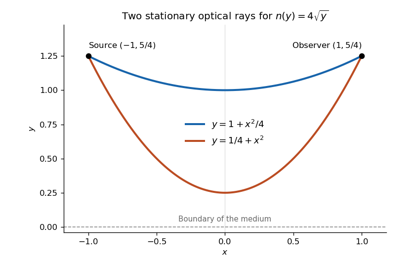
The original PDF places both endpoints at height ; the vertically stacked fraction can be misread in extracted text. The coefficient in the index is , multiplying .
For the optical-length integrand , the Beltrami identity applies because there is no explicit dependence. It giveswhere is constant. Therefore . The full Euler-Lagrange equation is , and combining these gives . This also excludes a constant curve, which would satisfy the squared first integral but not the full variational equation. Integration yieldsEqual endpoint heights at require . The height condition then becomes , or . Its two positive roots are and . Hence the two possible stationary rays areBoth stay in , have the required endpoints and satisfy the variational equation. These are the two optical rays in a square-root refractive-index profile. Fermat stationarity supplies two rays; it does not assert that both globally minimize travel time.

Take real admissible functions with finite , positive , and a self-adjoint domain for the Sturm-Liouville operator. Compactly supported variations avoid any boundary contribution at infinity. Formal self-adjointness givesFor , the quotient rule therefore givesVanishing for arbitrary variations requiresConversely an eigenfunction in the self-adjoint domain makes this variation zero. Multiplying its equation by and integrating also shows directly that its stationary quotient is .
Thus the stationary values are the admissible eigenvalues. Under the usual positive-weight, semibounded hypotheses the lowest is the global minimum, while higher eigenfunctions generally give saddle points. The assumption alone is not a complete domain specification for arbitrary : the required integrals and boundary form must exist. The rapidly decaying oscillator trials in part (b) meet these conditions.
Normalize the Gaussian trial first. The Gaussian integral givesIts second and fourth moments are and . Since , the kinetic term is . At the specified coupling, the energy is thereforeThe stationary condition isThe quadratic factor is positive for real , so the unique positive stationary width is . Also and diverges at both ends of , proving a global minimum within this trial family. Its value isThe associated Sturm-Liouville problem isHere , and . The Rayleigh-Ritz variational principle makes the exact lowest eigenvalue the minimum over all normalized admissible states. Restricting to Gaussians can only raise this minimum, hence . The inequality is strict because is not constant: the trial is not an exact eigenfunction. This is the Gaussian trial for a quadratic-plus-quartic oscillator.
Enlarge the trial space while retaining the optimized Gaussian. For example, usenormalize it and minimize the Rayleigh quotient over its coefficients, optionally optimizing too. This even trial space respects the even ground-state parity of the confining symmetric potential and adds independent shape freedom beyond a Gaussian width.
The original Gaussian remains included by setting the later coefficients to zero, so the optimized upper bound cannot increase. Finite-basis optimization is the Rayleigh-Ritz method, with matrix entries given by the Hamiltonian and overlap integrals. Increasing the basis size systematically improves the available approximation.
For any real coupling, the same normalized Gaussian family has energyIf , then as the negative term dominates the positive and terms. Each trial still has finite energy, is normalized and decays at infinity, but its energy tends to . ThereforeThis variational sequence makes the instability of the negative quartic potential explicit, without mistaking any local well near the origin for a global ground-state bound.
Articles were limited to the first 100 out of 185 total.
Articles by others on the same topic
There are currently no matching articles.