Original source: Released examination PDF, physical pages 347–350. All three note alternatives and both longer questions are treated.
Let be the transmission direction. An ideal linear polarizer projects the incident electric field onto this direction, so its Jones matrix isSince , the amplitude transmitted by a sequence of polarizers is the product of the projections between successive axes. Here the four directions are . After the first polarizer the unpolarized light input has intensity and is in linear polarization along . The transmission through a sequence of linear polarizers therefore follows from successive applications of Malus's lawThe relative angle between the rotating polarizers is , not . The first factor is an ensemble average over incident polarization: unpolarized light cannot be represented by a single deterministic Jones vector. Equivalently, its coherency matrix is ; the total matrix gives the same output intensity by the trace rule. The quasistatic optical-element approximation assumes the mechanical rotation is slow compared with the optical oscillation.
To first order in the applied fields, the carrier acceleration gives . The current density consequently obeys the first London equationTaking its curl and using Faraday's law yieldsFor an initially field-free, current-free preparation, the integration constant is zero. Equivalently, impose the second London equation appropriate to the Meissner state, . In the final static state, Ampère's law and then giveFor a planar half-space with a tangential surface field, the bounded solution isThe plasma-frequency form of London penetration depth therefore shows that an applied field is exponentially small several penetration depths inside the material.
The magnetic-history constant in an undamped plasma explains the required qualification. Undamped carrier motion alone fixes a time-independent value of ; it does not force that value to vanish. A perfect conductor can retain a pre-existing field. The additional London equation describes London screening independently of that arbitrary ideal-conductor history. The original London paper explicitly distinguishes its description from acceleration theory.[ref]
The electromagnetic equations of the supraconductor by Fritz London and Heinz London. pp. 71–74: acceleration equation, its integration freedom and the additional superconducting relation
wave phase labels the stage of a physical oscillation at a spacetime event. Two observers comparing the same event must identify the same crest, trough or intermediate stage: a change of coordinates cannot change the number of completed cycles between physically specified wavefronts. The continuous wave phase can therefore be treated as a Lorentz scalar, up to a common choice of wave phase origin. This does not assert invariance of the measured angular frequency, which is the rate of change of that wave phase along the observer's trajectory.
For Lorentz invariance of plane-wave phase, writeusing the metric with signature . The gradient transforms as a covector because is a scalar. Raising its index therefore gives the four-wavevector. Explicitly, substituting the inverse boost , givesThese are exactly the Lorentz transformation laws for . In vacuum, ; the Doppler effect and aberration of light are two consequences of transforming the same four-vector.
The Faraday effect rotates the plane of linear polarization when light propagates through a material with a magnetic field component along the ray. In the weak-field transparent regime,with a stated propagation and transverse-basis convention; is the Verdet constant. For a uniform longitudinal field and sample length , the magnitude is . A scalar intensity change without a corresponding polarization analysis would not establish this effect.
The microscopic field breaks the equivalence of the two circular polarization modes: the Lorentz force and the Zeeman shifts of optical transitions produce different susceptibilities for their opposite senses of rotation. A linearly polarized wave is an equal-amplitude superposition of these two modes. If their real refractive refractive indices are , their relative wave phase after the sample is . Recombination rotates the line byEqual transmitted circular amplitudes preserve linear polarization. Unequal absorption produces circular dichroism and generally elliptical polarization as well, so pure rotation is an approximation appropriate away from strong absorption.
A modern motivating experiment sends polarized laser light through a glass rod inside a solenoid, then through a rotatable analyzer onto a photodiode. Scan the analyzer first to calibrate its angular response. Driving the solenoid sinusoidally and recording the detector synchronously separates a small rotation signal from unsynchronized noise; the conversion to angle still requires the analyzer slope and the magnetic-field integral through the rod. A first-party William & Mary laboratory manual specifies this apparatus and measurement procedure.[ref]
Physics 251: Experimental Atomic Physics, Fall 2019. Faraday Rotation laboratory chapter, pp. 2–7: solenoid, glass rod, analyzer calibration and synchronized readout
Additional controls are equal-magnitude field reversals, zero-field readings before and after each pair, and a blocked-beam pickup test. The odd-in-field rotation is ; a fixed analyzer offset cancels. Heating, stressed-glass birefringence, source drift and field-dependent transmission need separate checks. A single reading near crossed extinction loses the sign because its leading response is quadratic; an analyzer near gives a linear small-rotation response.
Faraday rotation is nonreciprocal. With the magnetic bias held fixed, retracing the path adds rotation in the same laboratory sense rather than undoing it, unlike reciprocal natural optical activity. This permits an optical isolator with a Faraday rotator between appropriately oriented polarizers. One must compare the returned polarization in a consistently defined laboratory basis; merely reversing the sign of while retaining the old ray-basis convention gives an incorrect cancellation.
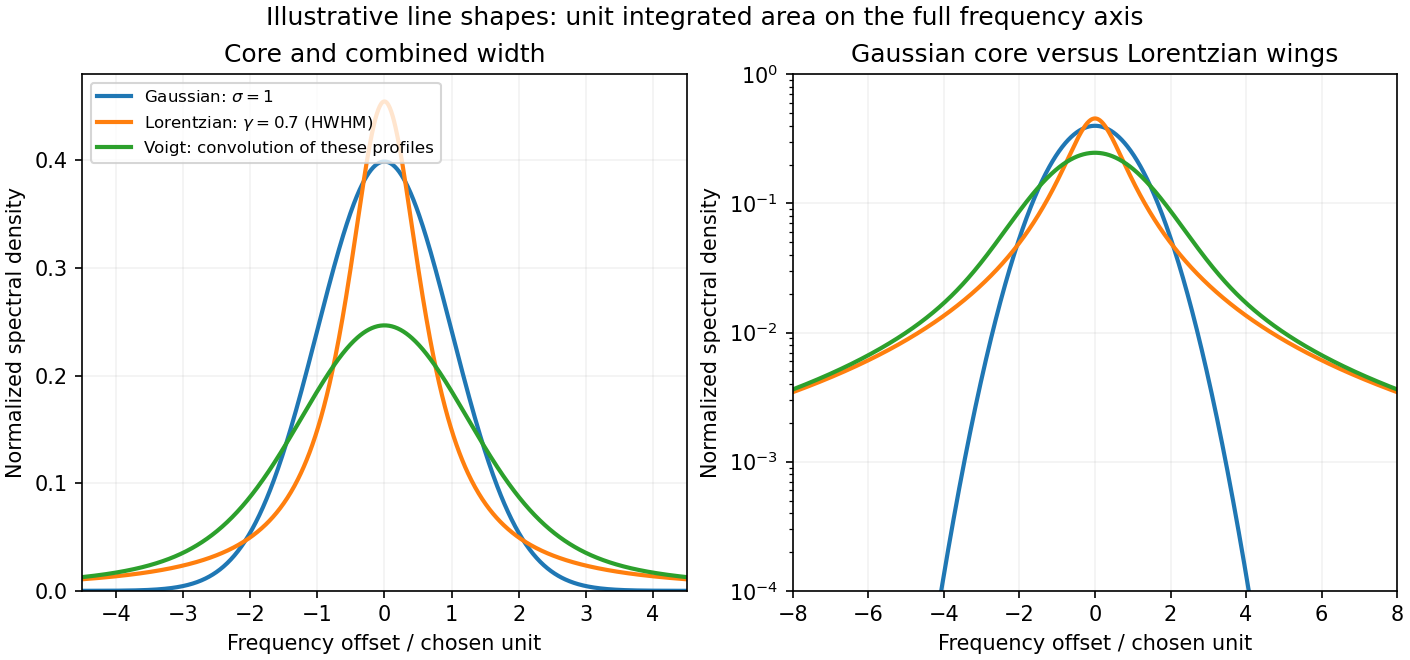
A spectral line has finite width when the emitted or absorbed field loses coherence, or when different emitters have different transition frequencies. It is useful to distinguish homogeneous spectral broadening of each emitter from inhomogeneous spectral broadening across the ensemble.
Finite lifetime and dephasing. For an upper-state population lifetime and a stable lower state, the radiating amplitude decays as . Its Fourier spectrum is Lorentzian, with full width at half maximumMore generally, an optical coherence time gives . Both level lifetimes and pure dephasing can contribute to . Distinguishing population lifetime from amplitude coherence time prevents the usual factor-of-two error.
Thermal motion. To first order in velocity, . A Maxwell-Boltzmann velocity distribution therefore produces a Gaussian profile, withThis is inhomogeneous doppler broadening: different velocity classes have different resonance frequencies. A distribution of bulk velocities can add further broadening, while a common bulk velocity shifts the line.
Interactions with the surroundings. Collisions can interrupt the dipole wave phase and perturb the energy levels, producing pressure broadening and shifts. In the impact approximation, approximately exponential wave phase relaxation produces a Lorentzian contribution; its rate increases with perturber density times an appropriate velocity-averaged collision cross section. Slowly varying electric microfields can instead produce non-Lorentzian Stark profiles. Neutral perturbers, charged perturbers and resonance interactions need not produce the same line shape. These mechanisms and the Gaussian thermal limit are distinguished in NIST's atomic-spectroscopy compendium.[ref]
Atomic Spectroscopy - A Compendium of Basic Ideas, Notation, Data, and Formulas by William C. Martin and Wolfgang Wiese. section 20, Spectral Line Shapes, Widths, and Shifts: Doppler and pressure broadening
Finite observation time limits coherence; transit-time broadening also occurs for particles crossing a narrow optical beam. Strong resonant excitation causes power broadening: for an ideal lifetime-limited two-level transition, with population decay rate and saturation parameter . Unresolved fine structure, hyperfine structure, isotope components, or spatially varying Zeeman and Stark shifts may look like a single broadened feature even though several frequencies are present.
The observed spectrum is additionally convolved with the instrument response. A Gaussian Doppler contribution convolved with Lorentzian homogeneous broadening gives a Voigt profile; their full widths do not generally add in quadrature. An informative experiment varies temperature, perturber pressure and excitation intensity separately, calibrates the spectrometer response with a narrower reference, and checks optical thickness or self-absorption. Extrapolation to weak excitation and low pressure helps isolate the lifetime contribution, while a Doppler-free technique is needed if velocity spread still dominates.
Both Thomson scattering and Rayleigh scattering can be understood as radiation from a dipole driven by the incident electric field. Their different frequency dependences come from the response of a free charge compared with a bound charge.
For a free particle of charge and mass , a harmonic field gives , hence . The radiated field contains two time derivatives of , cancelling the response's . The Thomson cross section is consequently independent of frequency in the classical low-recoil regime:For incident linear polarization with unit polarization , summing over outgoing polarizations gives . Radiation vanishes along the acceleration and is strongest perpendicular to it. Averaging an incident unpolarized light beam giveswhere is the scattering angle. Scattering through is fully linearly polarized perpendicular to the scattering plane for this ideal isotropic dipole model. The electron case dominates over equally charged heavier particles because the cross section scales as . recoil corrections become necessary when photon energy is no longer small compared with .
For a bound charge with natural frequency and damping rate ,Far below resonance, is approximately constant, soThis is Rayleigh scattering. It requires a scatterer small compared with the wavelength and, for the simple expression, an isotropic linear dipole response. Atoms, molecules and small dielectric particles provide examples. The stronger scattering of shorter visible wavelengths explains blue skylight; absorption and the nonuniform solar spectrum prevent treating that simple scaling as a complete color calculation.[ref]
Rayleigh Scattering by Richard Fitzpatrick. section 9.6, bound-charge response and low-frequency limit
For isotropic electric scatterers the normalized angular and polarization patterns are the same as in Thomson scattering. The frequency scaling distinguishes their limits: a free charge has a displacement proportional to , whereas a tightly bound charge has an approximately frequency-independent displacement. Near resonance, far outside the small-particle limit, or with anisotropic polarizability, the simple Rayleigh formula must be modified. In particular, the electric-only pattern must not silently be applied to a perfectly conducting sphere whose magnetic dipole response is also retained.
A scattering measurement should subtract stray-light and detector backgrounds, control scatterer density and optical thickness, and calibrate detector response and incident power when comparing wavelengths. A polarization analyzer at tests the dipole pattern; multiple scattering or unresolved nonisotropic contributions can reduce its polarization.
antenna quantities. radiation resistance represents emitted power by at the feed. It is not Joule heating in the antenna; a separate loss resistance accounts for that. antenna gain is the directional far-field intensity relative to an isotropic radiator supplied with the same input power:It includes radiation efficiency and equals antenna directivity only for a lossless antenna. antenna effective area is defined by the power available to a matched load, , for incidence from a specified direction and matched polarization. It need not equal a literal geometric collecting area.
Gain–area relation. To derive the antenna gain-effective-area relation, take a passive reciprocal antenna. Its electromagnetic reciprocity makes the receive pattern proportional to the transmit pattern; write . The normalization follows from thermal equilibrium. In the Rayleigh-Jeans law limit, blackbody radiation radiance per unit frequency per unit solid angle is for two polarizations. A single antenna polarization couples to one half, so the available incident noise power isThe open-circuit Johnson voltage spectrum of the antenna resistance is . A matched load receives half the open-circuit voltage, giving available power . In a lossless antenna at thermal equilibrium these powers agree; hence . Since ,The same efficiency factor multiplies receiving area and gain if reciprocal dissipative losses are included consistently. Impedance mismatch or polarization mismatch reduces delivered power further. The factor of two for thermal polarization modes and the factor of four between open-circuit voltage variance and matched-load power are separate effects.
Normalize the radar beam. Interpret the azimuth as signed about the beam centre at , so both sides of the narrow lobe are included. Put . To leading order in the small angular width, and the angular integrals can be extended over the real line:The Gaussian antenna beam solid angle gives the peak on the positive -axis consequently hasHere is power per solid angle, equal to in the far field. The leading neglected solid-angle correction is relative order .
Return using the supplied electric-dipole response. The electric-dipole radar cross section of a small conducting sphere determines this return. At target range , the incident intensity is . Write its root mean square electric field as , with . The induced electric dipole is . A dipole's angular radiation pattern, normalized by , gives . The backward direction is perpendicular to the induced dipole, so the supplied total dipole power givesThe received intensity is this angular power divided by . Using the monostatic radar equation, or directly multiplying by the receive area, givesThe receiver threshold is a voltage across the matched load, so the detectable power is , without another matching factor:This is the electric-dipole result following from the response data provided. It assumes , far-field propagation on each leg, alignment at the beam maximum and no attenuation or additional receiver losses.
Perfect-conductor qualification. perfect-conductor sphere dipole interference arises because the sphere also excludes the oscillating magnetic field. Solving the magnetic boundary problem gives in addition to the electric dipole. The magnetic polarizability of a perfectly conducting sphere follows from its induced surface currents.[ref]
Electromagnetic Fields and Energy by Hermann A. Haus and James R. Melcher. section 8.4, Example 8.4.3: magnetic dipole induced in a perfectly conducting sphere
In the backward direction the magnetic contribution has half the electric scattering amplitude and the same sign, so the returned intensity is of the electric-only value. Equivalently, the monostatic radar cross section is , rather than . Including both leading dipoles therefore givesBoth results have been distinguished because the supplied auxiliary data describe only the electric dipole, while the literal perfect-conductor boundary conditions also generate the magnetic one. The backward interference is a leading-order effect, not a higher-order correction in .[ref]Scattering of EM Waves by Michael Fowler. section Scattering by a Small Perfectly Conducting Sphere: electric and magnetic dipoles and backward interference
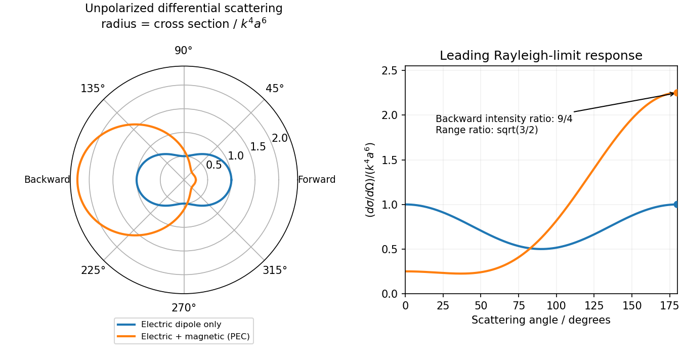
Original electric-only and electric-plus-magnetic small-sphere scattering comparison
. Details. Polarization under a boost. Lorentz invariance of normalized plane-wave polarization preserves the polarization ellipse's shape, handedness and degree of polarization when its transverse basis is carried to the aberrated ray. The propagation direction changes; equality of a fixed laboratory Cartesian pair of field components is not the appropriate comparison.
Rotate the axes so that a general incident vacuum plane wave has unit direction . Choose the transverse basis , , and arbitrary complex amplitudes . ThenPutting , the given transformation givesThe four-wavevector transforms with Doppler factor , givingIn the corresponding basis , , the transformed field isBoth components of the Jones vector acquire the same positive real multiplier. Their amplitude ratio and relative wave phase are unchanged, proving preservation of arbitrary linear, circular or elliptical polarization. All Stokes parameters scale by , so their normalized values and the degree of polarization are unchanged. An unpolarized light ensemble remains unpolarized under this single-ray boost. A mixture of different ray directions requires separate transformations and is outside this statement.
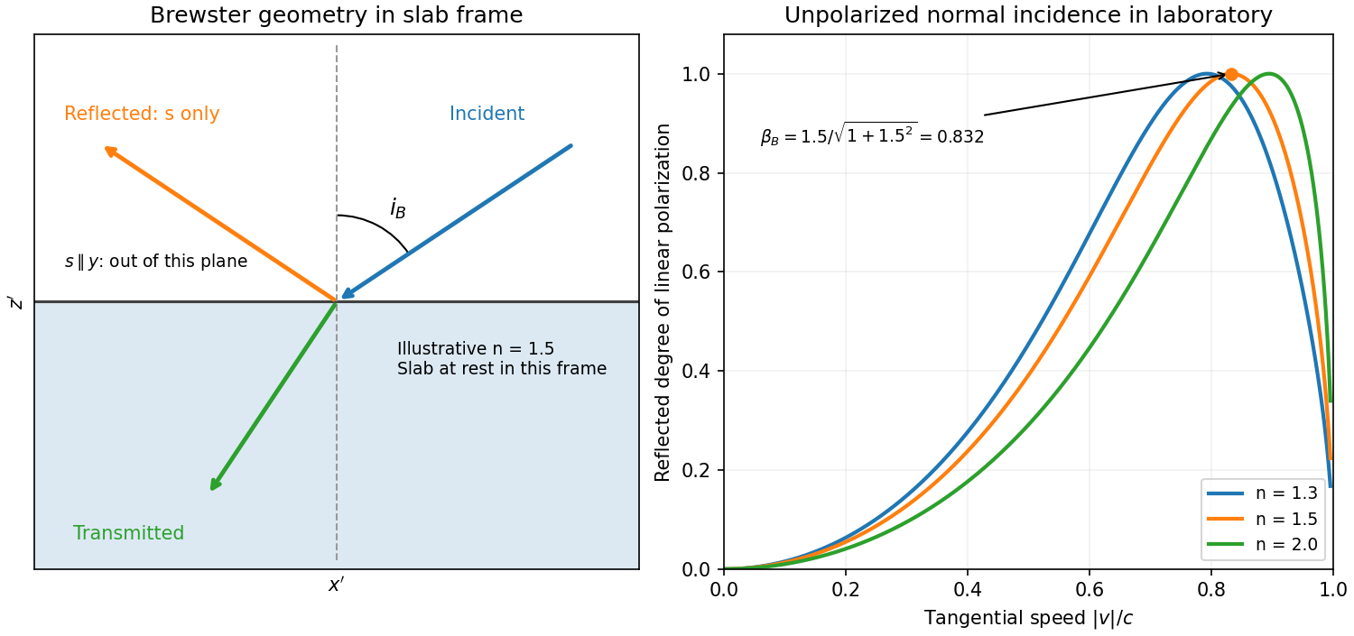
Reflection from the moving slab. Take the upper interface as , the material below it, and the incident ray along . This fixes the sign left implicit by “along the -axis”; choosing the opposite surface convention changes no result below. Treat as the real refractive index in the slab's rest frame, with unit relative magnetic permeability. In the laboratory,Transform to the slab rest frame:The incidence is now oblique, in the plane, at angle to the surface normal:The incoming ensemble remains unpolarized light. In this frame the ordinary stationary-interface Fresnel equations give the amplitude coefficients:For generic oblique incidence, and differ. Equal incident and intensities therefore produce unequal reflected intensities: the reflection is partially polarized. Its degree of linear polarization isThe inverse boost preserves this degree, so the same conclusion holds in the laboratory even though the laboratory incident ray is normal to the surface. The moving material cannot be treated as an isotropic stationary dielectric in that frame.
The reflected rest-frame wavevector is . Boosting back gives : the reflected laboratory ray is normal to the surface and has the incident frequency. There is no contradiction with the oblique rest-frame geometry. Translation tangential to a uniform interface does not itself introduce a moving normal mirror.
Complete linear polarization. For Brewster reflection from a tangentially moving dielectric, at Brewster's angle, and . Combining this with the aberration relation givesOnly the component is reflected. The plane of incidence in the slab frame is , so the reflected electric field is along , perpendicular to the slab velocity. Boosting this field back keeps its electric direction along . For example, the reflected rest-frame field has ; hence and .
This exact extinction assumes a transparent nonmagnetic dielectric with . At the reflected intensities are equal and the reflected beam is unpolarized. If , both reflection coefficients vanish and there is no reflected beam whose polarization can be assigned. With dispersion, evaluate at the shifted frequency ; the Brewster-speed equation is then implicit. absorption generally prevents a real incidence angle from making the complex exactly zero.


Articles by others on the same topic
There are currently no matching articles.