Past exam of the options II course of the University of Oxford / 2007 (AO2, XMAT 4304)

Options II, Honour School of Mathematics; Friday 22 June 2007, 2.30pm–5.30pm. The full twelve-page source, including the original identification diagram and all nineteen questions, is privately transcribed from original Part A bundle pages 20–31, supplied through the past-papers disclosure. No exact worked-answer advertisement was found in the bounded availability check. Printed formulas that are false as stated are retained in the transcription; the corresponding solutions explain their corrections.

Every nonzero vector can be extended to a basis, and the invertible map between two such bases carries the first vector to the second. The action is therefore transitive. Counting ordered bases givesThe stabilizer $H$ of one nonzero vector consequently has order $168/7=24$. There are three planes containing that vector, corresponding to the three lines of the two-dimensional quotient space. Adapted bases show $H$ acts transitively on these planes, so the stabilizer of one such plane has order $24/3=8$.

Let $Q$ be any subgroup of order eight. Its orbit lengths on the seven nonzero vectors are powers of two. Since their sum is odd, at least one orbit has length one. Fix such a vector $v$. The action on the three planes through $v$ likewise has a fixed plane $P$. Thus $Q$ is contained in the stabilizer of the flag $⟨v⟩\subset P$, and equality follows because that stabilizer already has order eight. The full group acts transitively on these flags, so all the subgroups are conjugate.

There are $7\cdot 3=21$ flags. To see they yield distinct subgroups, use the standard upper unitriangular matrices relative to an adapted basis. Their only common nonzero fixed vector is the first basis vector: varying entries in positions $(1,2)$ and $(1,3)$ forces the other two coordinates to vanish. On the quotient by that line, varying position $(2,3)$ leaves only the line of the second basis vector fixed. Hence this subgroup fixes exactly one full flag. Conjugation transfers uniqueness to each flag stabilizer, giving

An element is algebraic over $F$ if it is a zero of some nonzero polynomial in $F[x]$. An extension is algebraic if every element is algebraic. If $[K:F]=d<\infty$, the $d+1$ elements $1,\alpha ,\dots ,{\alpha }^d$ are linearly dependent over $F$, proving every $\alpha \in K$ is algebraic.

The converse fails for the algebraic closure $\overline{\mathbb{Q}}$ inside $\mathbb{C}$. All its elements are algebraic by definition, but it contains $2^{1/n}$ of degree $n$ for every positive integer $n$, since $x^n-2$ is irreducible by Eisenstein's criterion at two. A finite extension could not contain elements of unbounded degree, so this algebraic extension is infinite.

All sixth roots of unity lie in $\mathbb{Q}({\zeta }_6)$, with ${\zeta }_6=(1+\sqrt{-3})/2$. Its quadratic polynomial $x^2-x+1$ has no rational root, so

A primitive seventh root generates all seventh roots, so the splitting field is $\mathbb{Q}({\zeta }_7)$. Its minimal polynomial is the given irreducible cyclotomic polynomial $1+x+\cdots +x^6$. Therefore $\boxed{[K:\mathbb{Q}]=6}$.

A primitive eighth root satisfies ${\zeta }_8=(1+i)/\sqrt{2}$, while $i={\zeta }_8^2$ and $\sqrt{2}={\zeta }_8+{\zeta }_8^{-1}$. Thus $K=\mathbb{Q}(i,\sqrt{2})$. The real elements of $\mathbb{Q}(i)$ are rational, so it does not contain $\sqrt{2}$. The tower law gives

The cubic $x^3+x+1$ has no zero in ${\mathbb{F}}_2$, so is irreducible. Its quotient field has eight elements. Every nonzero element of that field satisfies $x^7=1$ by the order of its multiplicative group, so the polynomial splits there. It does not already split in the base field; a root of that irreducible cubic, which divides $x^7-1$, is needed. Hence

In characteristic two, repeated squaring gives $x^8-1=(x-1{)}^8$. There is only the root one, already in the base field. Thus $\boxed{K={\mathbb{F}}_2,[K:{\mathbb{F}}_2]=1}$. Repeated roots do not require a larger splitting field.

Wilson's theorem states that for a prime $p$, $(p-1)!\equiv -1(\mathrm{mod}p)$. For odd $p$, pair each nonzero residue with its multiplicative inverse. Only the self-inverse residues remain unpaired; $x^2=1$ in a field gives $x=\pm 1$. Their product is $-1$, proving the result. For $p=2$ the assertion is immediate.

If composite $n\ge 6$ is not the square of a prime, choose a prime divisor $p$ such that $p$ and $n/p$ are distinct. Both occur among the factors of $(n-1)!$, so their product $n$ divides it. In the remaining case $n=p^2$, $p\ge 3$, and the two distinct factors $p,2p$ both occur in the factorial and have product divisible by $p^2$. Thus the factorial is zero modulo every such composite $n$.

For prime $n$, Wilson's congruence makes the numerator sine squared equal ${\sin }^2(\pi /n)$, so its ratio is one. For composite $n\ge 6$, the numerator vanishes. The only exceptional composite in the sum is four; its ratio is ${\sin }^2(3\pi /2)/{\sin }^2(\pi /4)=2$. Therefore for $x\ge 4$ the sum counts the primes plus two, and subtracting two gives exactly the required prime count. All statements concern the integers $2\le n\le \lfloor x\rfloor$.

A coordinate transformation is a continuously differentiable bijection from the open set $U$ onto an open image, with continuously differentiable inverse. Equivalently one may specify a one-to-one continuously differentiable map whose Jacobian determinant is everywhere nonzero; the inverse function theorem gives the corresponding smooth inverse on its image.

The change-of-variables formula isFor an integrable $f$, the transformed function with its absolute-Jacobian factor is integrable as well. The absolute value is essential because the integral does not depend on whether the coordinate change preserves orientation.

Use $u=x-y$, $v=x+y$. It sends the diamond-shaped open square onto $(-1,1{)}^2$, and the inverse Jacobian has absolute determinant $1/2$. On this rectangle $|u|<1$ and $v+2>1$, so the original function is measurable, bounded by one and supported on a finite-area set, proving integrability. The transformed integral separates:The two one-dimensional integrals follow from the fundamental theorem of calculus; Fubini's theorem applies by the established integrability.

The dominated convergence theorem says that if measurable $f_n\to f$ almost everywhere and $|f_n|\le g$ for an integrable $g$, then $f$ is integrable, $\int |f_n-f|\to 0$, and consequently $\int f_n\to \int f$.

First derive Fatou's lemma from monotone convergence. For nonnegative $u_n$, the measurable functions $v_n={\inf }_{j\ge n}{u}_j$ increase to $\mathrm{liminf}{u}_n$, and $\int v_n\le {\inf }_{j\ge n}\int u_j$. Monotone convergence therefore yields $\int \mathrm{liminf}{u}_n\le \mathrm{liminf}\int u_n$.

Now $f$ is measurable and $|f|\le g$ almost everywhere, so is integrable. Apply Fatou's lemma to $u_n=2g-|f_n-f|\ge 0$, which converges almost everywhere to $2g$:The last integrals are nonnegative, so they tend to zero. Finally $|\int f_n-\int f|\le \int |f_n-f|\to 0$. This argument also works for complex-valued functions.

At each $x>0$, eventually $x<n$, and the stipulated power limit gives $f_n(x)\to e^{-x}\sin x$. At nonpositive $x$ the functions vanish. On their positive support,The supplied integrable exponential therefore dominates the sequence. Dominated convergence givesThe final improper integral is absolutely convergent, so agrees with its Lebesgue integral.

Compactness means every open cover has a finite subcover. Connectedness means the space cannot be written as the union of two disjoint nonempty open sets. The Hausdorff property means every two distinct points have disjoint open neighbourhoods.

True. Pull an open cover of $Y$ back through $f$. Surjectivity makes those inverse images cover $X$. A finite subcover of the compact space $X$ maps back to a finite subcover of $Y$. Thus a continuous image of a compact space is compact.

True. A separation of $Y$ into two disjoint nonempty open sets would pull back to a separation of $X$: continuity gives openness, and surjectivity gives nonemptiness. This contradicts connectedness of $X$.

True. Every singleton in a Hausdorff space is closed. Thus $f^{-1}(\{y\})$ is closed in $X$ by continuity. A closed subset of a compact space is compact, whether or not that compact space is Hausdorff. Hence every fibre is compact.

False. Take $X=[-1,1]$, $Y=[0,1]$ and $f(x)=x^2$, with their usual topologies. The domain is compact and connected, the codomain is Hausdorff, and the map is continuous and onto. But the fibre over one is $\{-1,1\}$, a disconnected two-point subspace.

False. Let $X$ be an indiscrete two-point space and $Y$ a one-point space. The constant map is continuous and onto; $X$ is compact because it is finite and connected because its only nonempty open set is the whole space. It is not Hausdorff, since its two points have no disjoint nonempty neighbourhoods. The one-point codomain is Hausdorff.

For the surjection $p$ to the set of equivalence classes, define a subset $V$ of the quotient to be open exactly when $p^{-1}(V)$ is open in $X$. Inverse images preserve the empty and full sets, arbitrary unions and finite intersections. Applying the topology axioms in $X$ proves this is a topology on the quotient, and it makes $p$ continuous.

The map need not be open. On $X=\mathbb{R}$, identify zero with one and leave every other point in its own class. The set $U=(-1/4,1/4)$ is open, but its saturation iswhich is not open in $\mathbb{R}$. Thus $p(U)$ is not open in the quotient topology. Continuity of a quotient map does not imply openness.

The surface is a Klein bottle. Here is a cell-count justification that keeps all the arrow directions. Name the corners of the first square $a,b,c,d$, beginning at its upper left and proceeding clockwise; name those of the second $e,f,g,h$ in the same way. The single-arrow gluing identifies $a$ with $e$ and $b$ with $h$. The triple-arrow gluing identifies $d$ with $h$ and $c$ with $g$. The first square's quadruple-arrow gluing identifies $b$ with $d$ and $c$ with $a$. The second square's double-arrow gluing identifies $e,f,g$ with one another. There are exactly two resulting vertex classes:There are four edge classes and two faces, so the Euler characteristic is $2-4+2=0$. Every edge is paired and the corner links close into circles, giving a compact surface without boundary; the cross-square identifications make it connected. It is nonorientable: the quadruple-arrow identification glues two boundary edges of the same square in the same boundary-traversal direction, so no orientation of that face can extend across the gluing. The classification of compact connected surfaces now identifies the nonorientable surface of Euler characteristic zero as the Klein bottle.

Geometrically, the internal identification in each square produces a Möbius band. The remaining single- and triple-arrow edges comprise their two boundary circles, which are glued together. The double of a Möbius band is another description of the same Klein bottle.

Differentiability at $a$ means that a linear map $L:V\to V_1$ satisfiesThis map is unique and is the total derivative $D{f}_a$. In finite dimensions linear maps are continuous.

The Frobenius norm is submultiplicative. Expanding the noncommuting cube givesThe last four terms have norm at most $3|A||H{|}^2+|H{|}^3=o(|H|)$. ThusIf $|C|<1$, the Neumann series ${\sum }_{j\ge 0}(-C{)}^j$ converges and is the inverse of $I+C$, as follows by multiplying its partial sums and letting the final power tend to zero. Its terms from degree two onwards have norm at most $|C{|}^2/(1-|C|)$. Hence $(I+C{)}^{-1}=I-C+O(|C{|}^2)$.

For invertible $A$, write $A+H=A(I+A^{-1}H)$. Whenever $|A^{-1}||H|<1$, this is invertible, proving the general linear group is open. The same expansion givesCompose this inverse derivative with the cube derivative, setting $B=A^{-1}$. The result isThe three terms cannot generally be combined into a scalar-style $-3A^{-4}H$, because matrix factors need not commute.

This is the cubic case of the Fréchet derivative of a negative matrix power.

Parametrize the surface by $r(x,\theta )=(x,y(x)\cos \theta ,y(x)\sin \theta )$, with $0\le \theta <2\pi$. Its tangent vectors are orthogonal, of lengths $\sqrt{1+y^{\prime 2}}$ and $y$. Thus the area element is $y\sqrt{1+y^{\prime 2}}dxd\theta$. Integrating over the angle gives

Discard the constant factor $2\pi$ when forming the Euler-Lagrange equation. For $F=y\sqrt{1+y^{\prime 2}}$ it becomesThe Beltrami identity, since $F$ has no explicit $x$ dependence, gives $F-y^{\prime }{F}_{y^{\prime }}=y/\sqrt{1+y^{\prime 2}}=C>0$. Combining with the differential equation yields $y^{\prime \prime }=y/C^2$. Its exponential solution has coefficients whose product is $C^2/4$, by $y^{\prime 2}=y^2/C^2-1$. Positivity therefore puts it in the formIts constants must satisfy $y_1=C\cosh ((x_1-K)/C)$ and $y_2=C\cosh ((x_2-K)/C)$. Depending on the endpoint data, these equations may have no solution or more than one. A constant function can satisfy a formal first-integral equation but fails the full Euler-Lagrange equation; it is not an extra extremal.

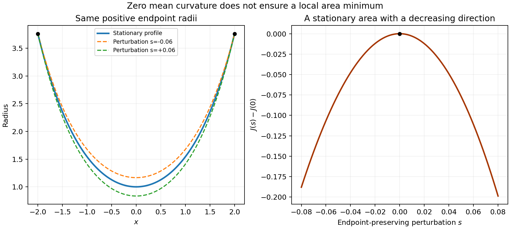
The functional is unbounded above. Let $y_0$ be the positive affine interpolant between the two endpoint values, and choose a smooth nonnegative function $\varphi$ that vanishes at the endpoints and is positive somewhere inside. The admissible curves $y_M=y_0+M\varphi$ satisfyThe claimed minimum conclusion does not follow and is false in general. A stationary point may have a negative second variation, even though the functional is unbounded above. Here is an explicit example within the allowed positive-graph class.

Take the stationary profile $y(x)=\cosh x$ on $[-2,2]$, and the endpoint-zero variation $\eta (x)=\cosh x-\cosh 2$. For sufficiently small perturbation parameter $s$, $y+s\eta$ remains positive and preserves both endpoint values. Put $C=\cosh 2$. Differentiating the area twice and integrating its mixed term by parts givesThis is strictly negative: the first term is less than $2\pi C$, while $(C+C^{-1})\tanh 2>\pi$. For example $e^2>7$ gives $C>7/2$ and $\tanh 2>24/25$, whose product already exceeds $\pi$. Thus nearby positive profiles have smaller area. This catenoid is not a local minimum.

The corrected conclusion is that any smooth positive minimizer, if attained, must have the catenoid form. That necessary condition is not sufficient, and existence or stability requires a separate argument.

Write $q=(x,X{)}^T$, $M=\left(\begin{array}{cc}a& b\\ b& c\end{array}\right)$ and $K=\left(\begin{array}{cc}\alpha & \beta \\ \beta & \gamma \end{array}\right)$. The linear equations are $M\ddot{q}+Kq=0$. A normal mode has all coordinates oscillating with one frequency and fixed relative amplitudes, $q=v\cos (\omega t+\phi )$. Its squared frequency solvesand its amplitude vector is a nonzero null vector of $K-{\omega }^{2}M$. The assumed distinct positive roots give two normal frequencies, their positive square roots.

For the rods let ${\theta }_1,{\theta }_2$ be their small inclinations from the downward vertical. To first order, ${\theta }_1=x/a$ and ${\theta }_2=(X-x)/(2a)$. The first rod has kinetic energy $m{\dot{x}}^2/6$. The second has centre-of-mass horizontal velocity $(\dot{x}+\dot{X})/2$ and angular velocity $(\dot{X}-\dot{x})/(2a)$, givingTogether these give $T=m(3{\dot{x}}^2+2\dot{x}\dot{X}+2{\dot{X}}^2)/6$. The centre-of-mass height changes giveproving the displayed quadratic Lagrangian.

Here $M=(m/3)\left(\begin{array}{cc}3& 1\\ 1& 2\end{array}\right)$ and $K=(mg/(2a))\left(\begin{array}{cc}6& -1\\ -1& 1\end{array}\right)$. Set $\lambda =2a{\omega }^2/(3g)$. The determinant equation reduces to $5{\lambda }^2-17\lambda +5=0$, soThe first row of the mode equation gives $X/x=(6-3\lambda )/(1+\lambda )$. The actual rod-angle ratio is thereforeIt is positive for the smaller root and negative for the larger root. Thus the low-frequency mode has the rods in phase, and the high-frequency mode has them out of phase. Using the rod-angle ratio is necessary because $X$ is the displacement of the end of the second rod, not that rod's inclination.

In vacuum, the source-free Maxwell equations are $\nabla \cdot E=\nabla \cdot B=0$, $\nabla \times E=-{\partial }_{t}B$ and $\nabla \times B=c^{-2}{\partial }_{t}E$. Put $\vartheta =\omega (t-z/c)$ and denote the field amplitude by $E_0$. The corresponding travelling-wave magnetic field isBoth divergences vanish because the fields have no longitudinal component and no dependence on the transverse coordinates. Direct differentiation gives $\nabla \times E=(\omega E_0/c)(\cos \vartheta ,\sin \vartheta ,0)=-{\partial }_{t}B$ and $\nabla \times B=(\omega E_0/c^2)(-\sin \vartheta ,\cos \vartheta ,0)=c^{-2}{\partial }_{t}E$.

Introducing potentials by $B=\nabla \times A$ and $E=-\nabla \varphi -{\partial }_{t}A$ automatically satisfies the magnetic-divergence and Faraday equations. The remaining Maxwell equations become equations for these potentials, with the usual gauge freedom. For $\omega \ne 0$ take $\varphi =0$ andDifferentiation verifies both potential relations.

The electromagnetic force is $Q(E+v\times B)$. Confinement also supplies a normal reaction force. For motion in a plane of constant $z$, both $v$ and $B$ are tangent to the plane, so their cross product is normal and is balanced by that reaction. It does not enter the in-plane equation $m\ddot{r}=Q{E}_0(\cos \vartheta ,\sin \vartheta )$.

At the fixed plane, the solution with no uniform drift isIt is circular, withOther initial data can add a constant drift velocity; the question only asks for the possibility of circular motion.

Orient the body boundary counterclockwise. The outward normal from the body satisfies $nds=(dy,-dx)$, so pressure givesFor steady irrotational flow, Bernoulli's equation makes $p+\rho |u{|}^2/2$ constant in the connected fluid region. Its constant contribution integrates to zero. Write $q=w^{\prime }=u-iv$. Impermeability says the velocity is tangent to the boundary, so $qdz=\bar{q}d\bar{z}$ there. Consequentlywhich proves Blasius' theorem with this contour convention.

The background stream function is the imaginary part of $w_0(z)=\alpha (z-c{)}^3$. Since its coefficients are real, the circle theorem givesIts derivative isIn $q^2$ the coefficient of $z^{-1}$ comes from the exponent pairs $(2,-3)$ and $(1,-2)$, including both orders. It is $36{\alpha }^{2}c{a}^4+36{\alpha }^2{c}^3{a}^2$. The residue theorem then givesThe vanishing transverse force also agrees with reflection symmetry about the real axis.

A material interface obeys ${\eta }_t+{\varphi }_{j,x}{\eta }_x={\varphi }_{j,y}$ at its actual height. Keeping only first-order terms and evaluating at the undisturbed interface gives ${\varphi }_{1,y}={\varphi }_{2,y}={\eta }_t$ at $y=0$. Linearized unsteady Bernoulli gives the pressure perturbation $-{\rho }_j({\varphi }_{j,t}+g\eta )$, after absorbing time-only constants into the potentials. Pressure continuity therefore givesFor $\vartheta =kx-\omega t$, choose potentials decaying away from the interface:They are harmonic and their normal derivatives equal $A\omega \sin \vartheta ={\eta }_t$ at zero. The dynamic condition reduces toIf the denser fluid is above, the squared frequency is negative. The corresponding perturbations grow or decay exponentially instead of oscillating: this is Rayleigh-Taylor instability, with growing rate $\sqrt{gk({\rho }_2-{\rho }_1)/({\rho }_1+{\rho }_2)}$ in the ideal model without surface tension.

The central limit theorem states that for independent identically distributed variables of finite mean $\mu$ and positive finite variance ${\sigma }^2$,For a continuous strictly increasing cumulative distribution function, its inverse is defined on $(0,1)$. Thus $\mathbb{P}(F(X)\le y)=\mathbb{P}(X\le F^{-1}(y))=y$ for $0<y<1$, proving the uniform law.

If $T=-\log (1-Y)$, then for $t\ge 0$, $\mathbb{P}(T\le t)=\mathbb{P}(Y\le 1-e^{-t})=1-e^{-t}$. Hence $f_T(t)=e^{-t}{1}_{(0,\infty )}(t)$, an exponential density of rate one. Its first two moments are one and two, by integration by parts, so $\mathbb{E}T=1$ and $\mathrm{Var}T=1$.

Although the original variables may have different distributions, their separate transforms $Y_k=F_k(X_k)$ are independent and all uniform. Consequently $T_k=-\log (1-Y_k)$ are independent identically distributed exponentials of rate one, and the statistic is exactlyThe stated central limit theorem therefore yields $\boxed{Z_n\stackrel{d}{\to }N(0,1)}$.

A Poisson process of rate $\lambda$ is a counting process starting at zero with independent stationary increments, with $N(t)-N(s)$ Poisson of mean $\lambda (t-s)$ for $t\ge s$, and right-continuous paths with unit jumps. Equivalently the small-interval probabilities are $\lambda h+o(h)$ for one event and $o(h)$ for two or more.

Independence of the two processes makes their joint increments over disjoint intervals independent. On an interval of length $h$, the sum of their independent Poisson increments has probability generating functionso it is Poisson with mean $(\alpha +\beta )h$. Simultaneous arrivals have probability zero, so the sum retains unit jumps. It is therefore a Poisson process of rate $\alpha +\beta$.

The first arrival times are independent exponential variables of rates $\alpha$ and $\beta$. For positive rates,

Stationarity at zero gives ${\pi }_0=q{\pi }_0+q{\pi }_1$, hence ${\pi }_1=(p/q){\pi }_0$. At one, ${\pi }_1=p{\pi }_0+q{\pi }_2$; substituting $p{\pi }_0=q{\pi }_1$ gives $q{\pi }_2=p{\pi }_1$. More generally the interior equations are ${\pi }_i=p{\pi }_{i-1}+q{\pi }_{i+1}$. Induction givesSince $p/q<1$, normalization of this geometric series givesThese probabilities satisfy detailed balance ${\pi }_{i}p={\pi }_{i+1}q$, including the boundary balance with the holding probability. Thus they do define a stationary distribution. Irreducibility then gives its uniqueness.

Apart from its multinomial coefficient, the likelihood is ${\prod }_{ij}{\theta }_{ij}^{n_{ij}}$. Maximizing its logarithm subject to $\sum {\theta }_{ij}=1$ gives $n_{ij}/{\theta }_{ij}$ equal to a common multiplier, which is $n$. Hence ${\hat{\theta }}_{ij}=n_{ij}/n$.

Under independence the log likelihood separates as ${\sum }_i{n}_{i\cdot }\log {\varphi }_i+{\sum }_j{n}_{\cdot j}\log {\rho }_j$. The two normalization constraints give ${\hat{\varphi }}_i=n_{i\cdot }/n$ and ${\hat{\rho }}_j=n_{\cdot j}/n$, so the fitted probabilities are $n_{i\cdot }{n}_{\cdot j}/n^2$. Therefore twice the difference of the maximized log likelihoods isThe unrestricted model has $rc-1$ free parameters and the independence model has $(r-1)+(c-1)$, leaving $(r-1)(c-1)=4$ degrees of freedom for the table. Under the null, the likelihood-ratio statistic is asymptotically chi-squared with four degrees of freedom. Since $25.192>18.467$, reject independence at the 0.1% significance level. This is evidence of association in the sampled variables; it does not by itself identify a causal direction.

Let $C$ be the clump size and put $q=e^{-\lambda t}$. The probability that all its members die, conditional on $C=n$, is $(1-q{)}^n$. Summing the geometric series givesSubtracting from one yields $\boxed{p(t,\lambda )=q/(1-\theta +\theta q)}$, for $0\le \theta <1$.

Assuming independent clumps and independent repeats, the combined likelihood is proportional to $p^R(1-p{)}^{N-R}$. For $0<R<N$ its unique maximizer is $\hat{p}=R/N$. The relation between $p$ and $q$ is one-to-one, with $q=(1-\theta )p/(1-\theta p)$. For $t>0$ this givesIf $R=N$, the estimate is the boundary value zero; if strictly positive rates are required, it is only a limiting supremum. If $R=0$, the likelihood approaches its supremum as $\lambda \to \infty$ and there is no finite estimate. These boundary cases explain when the printed logarithmic expression is finite.

The printed product omits the node with index zero. The correct cardinal polynomial isFor example, with two nodes zero and one, values zero and one, and both derivative data zero, the printed index range gives $L_1=1$ and its displayed interpolant is the constant one, which fails the value condition at zero. Thus the source formula cannot be proved literally.

With the corrected product, $L_k(x_j)={\delta }_{kj}$. For $j\ne k$, $L_k^2$ has a double zero at $x_j$, so both basis functions and their derivatives vanish there. At $x_k$, put $\ell =L_k^{\prime }(x_k)$. The value basis $H_k=L_k^2[1-2(x-x_k)\ell ]$ satisfies $H_k(x_k)=1$ and $H_k^{\prime }(x_k)=2\ell -2\ell =0$. The derivative basis $K_k=L_k^2(x-x_k)$ satisfies $K_k(x_k)=0$ and $K_k^{\prime }(x_k)=1$. Both have degree at most $2n+1$. Consequentlyhas every prescribed value and derivative, proving membership in the interpolation class after the required index correction. This corrected Hermite interpolant is used in the following parts.