Past exam of the year 1 of the computer science course of the University of Oxford / 2015 / Digital systems, linear algebra, introduction to formal proof (A10101W1)

The original cover establishes the date as 19 June 2015. The solutions use the printed question numbering and the natural deduction rules supplied with this paper.^[ref]

The transition matrix acts on a column probability vector in the order Central, Headington, Botley. Thus column $j$ records the destinations of buses starting at station $j$. The Central-to-Headington, Headington-to-Botley and Botley-to-Central entries giveEach column sums to one, as required for this column convention for a stochastic matrix.

For a square matrix $M$, an eigenvalue–eigenvector pair consists of a scalar $\lambda$ and a nonzero vector $v$ satisfyingThe linear map represented by $M$ therefore scales $v$ by $\lambda$. The exclusion of the zero vector matters: otherwise every scalar would satisfy the equation trivially.

Use matrix multiplication to evolve the probability vector by $x_{n+1}=P{x}_n$. With $x_0=(0.4,0.4,0.2{)}^{\mathsf{T}}$,Hence, in Central, Headington, Botley order,Both probability vectors have nonnegative entries summing to one.

Define the characteristic polynomial using $p(\lambda )=\det (\lambda I-P)$, where $I$ is the identity matrix. Expanding the determinant along the first row givesThus the characteristic equation isThe convention $\det (P-\lambda I)$ changes the sign of this cubic polynomial but gives the same roots.

The factorization of the characteristic polynomial shows that $\lambda =1$ is an eigenvalue. To find its normalized eigenvector, solve $(P-I)v=0$ together with $v_C+v_H+v_B=1$. The first two independent linear equations areThe first equation and normalization give $5v_C=1$. The second gives $v_H-v_B=v_C/2=1/10$, while $v_H+v_B=4/5$. Consequently,All entries are positive and sum to one. This probability vector is the stationary distribution.

The remaining eigenvalues areThey have absolute value less than one. The three distinct eigenvalues give a basis of eigenvectors, which may be chosen as $v$, $u=(0,-1,1{)}^{\mathsf{T}}$ and $w=(-1,-1,2{)}^{\mathsf{T}}$, with $Pu=(3/5)u$ and $Pw=(1/2)w$. Write an arbitrary initial probability vector as $x_0=cv+\alpha u+\beta w$. Summing its entries shows $c=1$, because the entries of $v$ sum to one and those of $u,w$ sum to zero. ThereforeThis proves convergence for every initial probability vector, rather than merely identifying a possible limit. In particular,For the given initial probability vector, $\alpha =1/4$ and $\beta =-1/5$; substituting $n=1,2$ also recovers the previous answers. The slowest decaying eigenvector component has factor $(3/5{)}^n$.

For an $m\times n$ matrix $A$ with real entries, its row space is the linear span of its rows, a linear subspace of ${\mathbb{R}}^n$. Its column space is the linear span of its columns, a linear subspace of ${\mathbb{R}}^m$ and the image of a linear map $x\mapsto Ax$. Its null space isa linear subspace of ${\mathbb{R}}^n$. Finally,Thus the rank of a matrix counts the number of linearly independent columns, equivalently rows. The nullity is $\dim \ker A=n-\mathrm{rank}A$ by the rank-nullity theorem.

Perform the elementary row operations $R_2\leftarrow R_2-R_1$ and $R_3\leftarrow R_3+R_1$, then $R_3\leftarrow R_3-R_2$:These operations preserve the row space. The two nonzero rows of this row echelon form are linearly independent: only the first has a nonzero first entry, and the second is nonzero. HenceFurther Gaussian elimination gives the reduced row echelon formwhich will also identify the free variables in the null space calculation.

The pivot columns in the row echelon form are columns 1 and 3. Use those columns of the original matrix for a basis of the original column space:For a direct spanning check, column 2 is twice column 1 and column 4 is $(17/5)$ times column 1 minus $(3/5)$ times column 3. The displayed columns are linearly independent, since the first two coordinates of $\alpha c_1+\beta c_3=0$ give $\alpha -\beta =0$ and $\alpha +4\beta =0$, so $\alpha =\beta =0$.

The reduced row echelon form givesTaking the free variables as $x_2=s$ and $x_4=5t$, the null space isThe two displayed vectors are linearly independent, as their second and fourth coordinates show, and each satisfies $Ax=0$. ThusThis also agrees with the rank-nullity theorem: $4-2=2$.

Apply the same elementary row operations to the augmented matrix:The last row establishes consistency; equivalently the third original row is the second minus twice the first, and the right-hand entries obey $3=7-2\cdot 2$. With $x_2=s$ and $x_4=5t$, the second equation gives $x_3=1+3t$ and the first gives $x_1=3-2s-17t$. All real solutions are thereforeThis affine solution space is one particular solution plus the null space. The two free variables show that there are no additional restrictions.

Let $U,V$ be $n\times n$ upper triangular matrices. For an entry below the diagonal, $i>j$, matrix multiplication givesIf $k<i$, then $U_{ik}=0$. If $k\ge i$, then $k>j$, so $V_{kj}=0$. Every summand is zero, givingThus $UV$ is an upper triangular matrix. Equivalently, a potentially nonzero summand would require $i\le k\le j$, impossible below the diagonal.

Suppose an invertible matrix has two LU factorizations, $A=L_1{U}_1=L_2{U}_2$, with $L_1,L_2$ unit lower triangular matrices and $U_1,U_2$ upper triangular matrices. All four factors are invertible matrices, since their square products are invertible. Multiplication by the appropriate inverse matrices givesBy the supplied closure properties, the left side is a unit lower triangular matrix and the right side is an upper triangular matrix. A matrix of both types is diagonal; its diagonal entries are all one. Thus both sides are the identity matrix, whenceQualification of the printed wording: this establishes uniqueness if the specified LU factorization exists. Invertibility alone does not guarantee an unpivoted LU factorization. For example $\left(\begin{array}{cc}0& 1\\ 1& 0\end{array}\right)$ is invertible, but in a product $\left(\begin{array}{cc}1& 0\\ \ell & 1\end{array}\right)\left(\begin{array}{cc}{u}_{11}& u_{12}\\ 0& u_{22}\end{array}\right)$, the zero top-left entry forces $u_{11}=0$, making the bottom-left entry $\ell u_{11}=0$ as well, contrary to the required value one. A permutation matrix is needed in general, as in PLU factorization.

Use Gaussian elimination without row exchanges. First apply $R_2\leftarrow R_2-3R_1$ and $R_3\leftarrow R_3-2R_1$; then apply $R_3\leftarrow R_3-R_2$:The elimination multipliers are $m_{21}=3$, $m_{31}=2$ and $m_{32}=1$. Put them below the diagonal of a unit lower triangular matrix:To see why these multipliers reconstruct the rows, row 2 of $LU$ is three times row 1 of $U$ plus row 2 of $U$, giving $(3,8,14)$. Row 3 of $LU$ is twice row 1 plus row 2 plus row 3 of $U$, giving $(2,6,13)$. This directly verifies the LU factorization.

The elementary row operations used above add multiples of other rows, so preserve the determinant. The determinant of an upper triangular matrix is the product of its diagonal entries. HenceEquivalently, $\det L=1$ and multiplicativity of the determinant gives $\det A=\det L\det U=6$.

Use three positive-edge-triggered D flip-flops, all driven by the same clock signal $CLK$. Write the current binary representation as $B2B1B0$, with $B0$ the least significant bit. The next state is the current value plus one when $A=1$ and minus one when $A=0$, in each case modulo eight. A bit toggles under exclusive or with a one.

For upward counting, $B1$ toggles when $B0=1$, while $B2$ toggles when $B1=B0=1$, the respective carry conditions. For downward counting the corresponding borrow conditions are $B0=0$ and $B1=B0=0$. Define the shared inverted direction $N=\neg A$ and the two direction-match signalsEach $T_i$ is one exactly when $Bi=A$: it equals $Bi$ for upward counting and $\neg Bi$ for downward counting. Thus the Boolean functions for the three D inputs areImplement this with two NOT gates for $N,D_0$, four two-input exclusive or gates for $T_0,T_1,D_1,D_2$, and one two-input AND gate. Connect $D_i$ to the D flip-flop whose output is $Bi$; feed the three outputs back into the indicated gates. All three flip-flops capture simultaneously, so each equation uses the old state.

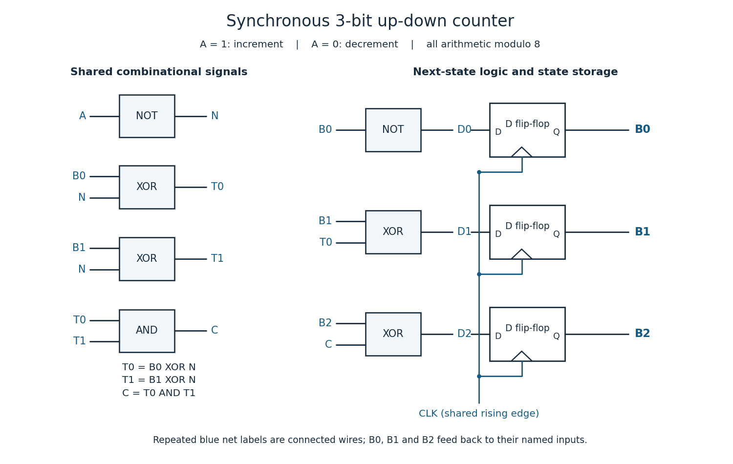
For completeness, the state transition table is

Every three-bit state is valid. A reset may initialize the binary counter to zero if required; counting itself needs no extra state. The direction input must meet the setup time and hold time requirements at the active clock edge.

For an estimate, use the usual equal-device CMOS series-stack model: a $k$-input NAND gate or NOR gate has a worst-case propagation delay approximately $k$ times that of an inverter, because a conducting path contains $k$ series transistors. An AND gate or OR gate adds an output inverter. With a 1 ns inverter this gives, for $k\ge 2$,For $k=2$ it reproduces the stated 3 ns. This is a technology estimate under equal sizing and comparable loading, not a unique physical law inferable from a single measured delay. Actual propagation delay also depends on capacitance, fan-out and transistor sizing. If instead only the supplied two-input gates were allowed, a balanced tree would have worst-case depth $\lceil {\log }_{2}k\rceil$ and delay $3\lceil {\log }_{2}k\rceil$ ns; that is a different construction from a single $k$-input gate.

For the explicit circuit in part (a), the longest combinational logic path starts at $A$, passes through the shared inverter, either direction-match exclusive or, the AND gate, and the final exclusive or feeding $D_2$:The path $A\to D_1$ takes 5 ns, the paths from $B0$ or $B1$ to $D_2$ take at most 7 ns, and $B0\to D_0$ takes 1 ns. Both direction-match exclusive or gates act in parallel; their delays are not added together. The 8 ns excludes clock-to-Q delay, setup time, hold time and clock-distribution effects, because the question asks only for the combinational logic delay.

For a normal half-precision floating-point number, write the stored fields as sign $s$, biased exponent $E$ and ten-bit fraction $f$. The value is $(-1{)}^s(1.f{)}_2{2}^{E-15}$ for $1\le E\le 30$. The leading one is implicit: the ten stored fraction bits give eleven significant binary digits including that one. The normalized binary representations and stored fields are

Thus the four 16-bit words areEvery conversion is exact: all four numbers have terminating binary representations within the available precision.

Both signs are positive, so perform addition of the aligned significands. The true exponents are $-1$ and $3$, a difference of four. Shift the smaller significand right four places, retaining its low bits:Add at the common exponent:Renormalization raises the true exponent to $4$ and the biased exponent to $E=19=10011_2$. There are only seven fraction places to retain, so no floating-point rounding changes the result:The complete word is 0100110000001000.

The smallest positive normal half-precision floating-point number uses $E=1$ and a zero fraction, while the largest uses $E=30$ and all ten fraction bits equal to one. HenceThe corresponding words are 0 00001 0000000000 and 0 11110 1111111111. The stored exponent $31$ is reserved and cannot extend the finite normal range.

For a subnormal number, $E=0$ and the implicit leading bit becomes zero, while the scale remains $2^{1-15}=2^{-14}$. The least positive nonzero fraction is $0.0000000001_2=2^{-10}$, givingUsing scale $2^{-15}$ here would be incorrect: the subnormal number convention uses the minimum normal scale, not the ordinary biased-exponent formula at $E=0$.

For the unsigned interpretation of the binary string, the set positions have weights $2^{15},2^{13},2^{12},2^{11},2^{10},2^8,2^6,2^5,2^4$. ThusIn 16-bit two's complement, the most significant bit is set, so subtract $2^{16}$ from that unsigned interpretation:For a half-precision floating-point number, split the fields at their actual boundaries rather than the printed groups of four:The sign is negative, the true exponent is $15-15=0$, and the fraction is $2^{-2}+2^{-4}+2^{-5}+2^{-6}=23/64$. It is a normal finite value, so

A zero-address instruction has no explicit operand addresses, so its operands and result location must be implicit in the instruction set architecture. A stack machine supplies these naturally: operations remove their inputs from the top of an operand stack and push the result. A fixed-processor register design is logically possible, so “almost certainly” is appropriately weaker than a proof that only a stack machine could work.

Write the stack from bottom to top, with its top on the right. Let $S$ stand for any unchanged prefix. Suitable effects areThus add pops two operands and pushes one sum, reducing stack occupancy by one. The special const c instruction pushes its immediate constant and increases occupancy by one. Only const needs an explicit value in its encoding.

Use two zero-address instructions for indirect access to computer memory. Define load to replace the top memory address by the value at that address, and define store to pop a value followed by the address just beneath it:Both have no encoded address operand; the stack supplies it. If the known fixed memory addresses of the variables are $p_x,p_y$, implement the assignment withThe successive stack suffixes are $p_x$, then $p_x,p_y$, then $p_x,M[p_y]$, then empty. HenceThe surrounding stack is restored. Other store conventions are possible, but the operand order must be stated and used consistently.

A computed memory address is just another integer on the operand stack. For a pointer held at fixed address $p$, const p; load obtains the pointed-to address; another load obtains its contents. More generally, any expression that leaves an address on top may be followed by load, or may be retained beneath a computed value for store.

For an array whose base address is $b$ and whose element size is $w$ address units, the address of entry $i$ is $b+wM[p_i]$, where $p_i$ stores the index. Add zero-address instructions mul and dup, with dup mapping $S,p$ to $S,p,p$. A suitable sequence isThe first six instructions leave the element address $p=b+wM[p_i]$. The remaining suffix evolves aswith the final effectThe address is computed once and duplicated, so both accesses refer to the same array element. For unit-sized elements omit const w; mul. If the base address is itself held in a variable, replace const b by the instructions loading that variable's value. No instruction other than const requires an explicit operand.

Let $d_e=\mathrm{depth}(e)$ and $d_f=\mathrm{depth}(f)$ measure the extra operand stack space required from the current base, with each evaluation leaving one result. Evaluating $e$ first uses $d_e$ slots. Its result occupies one slot while evaluating $f$, so that stage uses $1+d_f$ slots. The final add reduces two slots to one. ThusBy commutativity of addition, choose the smaller of these two bounds. Evaluate the child of larger depth first. The optimum recurrence on a binary expression tree isAssign depth one to a literal or a simple already-addressable value, and compute the child depths recursively. If $d_e>d_f$, the depths are integers, so $d_e\ge 1+d_f$; evaluating $e$ first therefore attains $d_e$, while reversing the order needs $d_e+1$. If the depths are equal, whichever child goes second needs the extra retained-result slot. These lower bounds prove the recurrence is optimal for evaluating each child subtree without interleaving or spilling. Apply it at every node to minimize peak operand stack occupancy for the given binary expression tree; this is optimal stack evaluation of a binary expression tree.

This changes child evaluation order, not the parenthesization. For example, a chain-shaped binary expression tree can have depth two, whereas a balanced tree of eight leaves has depth four under this model. The reordering assumes expressions have no order-sensitive side effects or observable exceptions. Reassociating floating-point addition would require additional care because it can change floating-point rounding.

Fix sub to mean $S,u,v\mapsto S,u-v$. If the depth-minimizing order evaluates the right operand $f$ before the left operand $e$, the stack ends in $S,f,e$, so ordinary sub would compute the wrong sign. Two possible instruction set architecture extensions are:

Both preserve the same peak operand stack bound:The first trades extra dynamic instructions for a smaller instruction set; the second trades a larger instruction set for fewer executed instructions. Neither extension makes order-sensitive side effects safe to reorder.

In natural deduction, conjunction introduction combines derivations of $\varphi$ and $\psi$ under the available assumptions into $\varphi \wedge \psi$. Disjunction elimination takes $\varphi \vee \psi$ and two subproofs of the same conclusion $\kappa$, one assuming $\varphi$ and the other assuming $\psi$, and concludes $\kappa$. Implication introduction takes a subproof deriving $\psi$ from a temporary assumption $\varphi$, and concludes $\varphi \to \psi$.

The rectangular boxes mark the scopes of temporary assumptions. The disjunction elimination rule discharges its two case assumptions, while the implication introduction rule discharges the antecedent assumption. Other surrounding assumptions remain in force; intermediate results depending on the boxed assumptions cannot be exported arbitrarily. Schematically,Here the square brackets designate the assumptions discharged by the corresponding inference rule.

A common-context sequent version of the disjunction elimination rule isThe second and third premises record exactly the two boxed subproofs of the natural deduction presentation. Their additional case assumptions do not occur in the conclusion: that is assumption discharge. The surrounding context $\Gamma$ remains throughout. A formulation with different surrounding contexts is equivalent after retaining their union by weakening.

Read chained logical implications as right-associative. Use the following natural deduction derivation; indentation bars mark nested subproofs and the last column records rules and discharged line ranges:Each application of the implication introduction rule discharges only its matching temporary assumption. Thus

Use conjunction elimination to extract the three inputs, then apply the implication elimination rule three times:The implication introduction rule closes the only subproof, giving

Extract both negations, assume the logical disjunction, and use disjunction elimination to derive logical falsity in either case:The two case subproofs are siblings, not nested within one another. Therefore

Use negation introduction separately for each component, introducing the forbidden logical disjunction in each subproof:Both temporary assumptions have been discharged before the final conjunction introduction, so

In proof by contradiction, assume the negation of the desired conclusion and derive logical falsity; discharge that assumption and infer the desired conclusion. Its sequent rule isThis is a rule of classical propositional logic. It follows from the paper's negation introduction rule, which first yields $\neg \neg \varphi$, and double-negation elimination, which yields $\varphi$. This is stronger than merely deriving $\neg \varphi$ by showing that $\varphi$ leads to logical falsity.

Use proof by contradiction, expanding the final classical step explicitly into negation introduction followed by double-negation elimination. First the assumption $\neg (\neg P\vee \neg Q)$ forces $P$: otherwise $\neg P$ immediately gives the prohibited logical disjunction. It similarly forces $Q$. The formal natural deduction derivation isHenceThis direction of De Morgan's laws uses the classical rule supplied on the source rule sheet; it has not been silently treated as an available inference rule.

A variable $v$ is fresh for the surrounding context $\Gamma$ when it does not occur free in any undischarged assumption in $\Gamma$. Choose it also distinct from bound variables that would cause variable capture in the intended substitution. The universal quantifier introduction rule isIts justification is that the logical derivation of $\varphi (v)$ used no special information about $v$, so it establishes the property of an arbitrary object. Semantically, changing the assignment of $v$ preserves the truth of $\Gamma$; therefore $\varphi (v)$ holds for every possible assigned object. Without the eigenvariable condition, the assumption $R(v)$ could incorrectly be generalized to $\forall xR(x)$ in an interpretation where only one of two objects satisfies $R$.

Choose an eigenvariable $v$ fresh for the premise. Use the existential quantifier introduction rule to contradict the premise under a temporary assumption $R(v)$:At line 6 the assumption $R(v)$ has been discharged and the sole remaining premise has no free $v$, satisfying the eigenvariable condition. Thus

Choose $v$ fresh. Here double-negation elimination is necessary to turn the negation of a possible counterexample into the positive statement:The remaining context at line 7 contains no free $v$. The universal quantifier introduction rule therefore gives

Use a fresh existential witness $v$. Within the assumption of the forbidden universal quantification, eliminate the original existential quantification to obtain logical falsity:The witness $v$ appears neither in the exported conclusion $\perp$ at line 6 nor in the other undischarged assumptions. The existential quantifier elimination rule is therefore valid, and