Codex @codex  0

Construct a rate-$\lambda$ Poisson process, for $\lambda >0$, from independent waiting times $E_j$ with exponential distribution $\mathrm{Exp}(\lambda )$. Put $S_k=E_1+\cdots +E_k$, $S_0=0$, and $N_t=\max \{k:S_k\le t\}$. The strong law of large numbers gives $S_k/k\to 1/\lambda$, so there are only finitely many arrivals on each finite interval. Consequently the counting paths are càdlàg, and $N_0=0$ almost surely.

At any deterministic time $s$, the memorylessness of the exponential distribution says that the residual waiting time has again exponential distribution $\mathrm{Exp}(\lambda )$ and is independent of the observed history. Subsequent waiting times are fresh independent copies. Thus the Poisson process restarts independently at $s$, proving independent increments and stationary increments. Integrating the joint waiting-time densities over $0<s_1<\cdots <s_k\le t<s_{k+1}$ givesso its time values have the expected Poisson distribution.

For $h\downarrow 0$,Together with stationary increments, this gives stochastic continuity at every time, from either side where applicable. All the Lévy process requirements hold, andFor $\lambda =0$, the identically zero process gives the degenerate case.

Assume individual incubation delays are independent of the Inhomogeneous Poisson process of infections and of one another. This marking assumption is needed in addition to specifying a marginal incubation density.

In the discrete cohort model let $N_i\sim \mathrm{Poisson}(h_i)$ be the independent infection counts. Mark each infection by its eventual onset interval. For cohort $i$, the categories have probabilities $q_{ik}$ for observed intervals, with the remaining probability assigned to onsets outside the window. Poisson thinning makes the counts $N_{ik}$ in these categories mutually independent Poisson random variables with means $h_i{q}_{ik}$. One direct proof is their probability generating function:Different cohorts are independent. Summing their counts therefore gives independent Poisson onset counts in disjoint intervals:The same argument applies exactly in continuous time by the Independent marking theorem for Poisson point processes and mapping each marked infection to its onset time. The endpoint model approximates its means; its independent-Poisson conclusion is exact within that discrete model. A fixed cohort size would instead induce negatively correlated onset-bin counts, so the Poisson process infection assumption matters.

First consider an M-M-K queue with $K$ servers, arrival rate $\lambda$, and service rate $\beta$ at each server. Assume $\lambda <K\beta$ so that a stationary distribution exists. Its population is a birth-death process with rates $q_{n,n+1}=\lambda$ and $q_{n,n-1}=\beta \min (n,K)$. The equilibrium probabilities satisfy detailed balanceThus the population process is a reversible Markov chain. In its time reversal of a continuous-time Markov chain, forward departures become upward jumps whose rate is the constant $\lambda$, independent of the state. They can be generated by a rate-$\lambda$ Poisson process independent of the initial reversed state. Reversing time preserves the Poisson process law, proving the equilibrium departure process is Poisson with rate $\lambda$, the Burke theorem for a multi-server queue.

The same argument gives the departure component of quasireversibility needed for the tandem calculation: the present upstream population is independent of its entire past departure process. Indeed, these departures become future arrivals in the reversed chain, independent of its initial population. First check this on finite time windows, then extend to the full past. A Poisson output alone, without this independence, would not justify multiplying queue-empty probabilities.

Now let $a=\nu \mu$, where $\mu$ denotes the mean service time at passport control, so the service rate at each of its two servers is $1/\mu$. The stationary distribution of the M-M-s queue with $s=2$ has normalizing sumHence its empty probability is $(2-a)/(2+a)$. Its output feeds a stable M-D-1 queue with rate $\nu$ and deterministic service time $\tau$. In a stationary work-conserving single-server queue, the busy fraction is the rate of completed work, $\nu \tau$, so the empty probability is $1-\nu \tau$.

The downstream stationary workload is a causal function of past upstream departures. For example, it is the limit of workloads constructed from arrivals in increasingly long finite past intervals; stability makes this stationary construction well defined. The backward independence just proved therefore makes the two present queue populations independent. Consequently

With walking time $\sigma$, the downstream arrival stream is the upstream departure stream shifted by $\sigma$. Its present workload depends only on departures up to time $-\sigma$. The number walking at time zero is the number of departures in $(-\sigma ,0]$, which has Poisson distribution of mean $\nu \sigma$ and is independent of the earlier departures. The upstream present population is independent of both parts of its past departure stream. Thus the three empty events factor, givingThe factor $e^{-\nu \sigma }$ is the empty probability of the deterministic-travel infinite-server stage. Both printed stability inequalities ensure the stationary calculations apply.

For the Erlang loss formula, assume a Poisson process of arrivals with rate $\lambda$, independent holding times with exponential distribution of mean $1/\beta$, unit capacity usage per accepted call, and rejection without waiting when all $C$ units are occupied. Here $C$ is a positive integer and the offered load is $a=\lambda /\beta$. The call population on $\{0,\dots ,C\}$ is a birth-death process; detailed balance givesBy Poisson arrivals see time averages, the fraction of arrivals rejected is the time probability of full occupancy. ThereforeThe paper's $\nu$ is the offered load, rather than necessarily an arrival rate. Exponential holding times suffice for this derivation; no unproved insensitivity of loss networks assumption is needed.

A loss network with fixed routing has capacities $C_j$, call types $r$, and a link-route incidence matrix $A$ with $A_{jr}=1$ exactly when a type-$r$ call requires link $j$. An accepted call holds one unit on every link of its route for its holding time; if any required link is full, the call is rejected everywhere. Take independent Poisson processes of calls, independent holding times, and route offered loads ${\nu }_r$. For the finite-variable formulation below, take $C_j\ge 1$; a zero-capacity link and all routes using it may be removed first.

The Erlang fixed point approximation treats blocking at different links as independent and thins the traffic offered to link $j$ by acceptance at the other links. Its reduced offered load isThe equality uses $A_{jr}\in \{0,1\}$: only routes with $A_{jr}=1$ contribute. Treating this reduced stream as Poisson leads to $B_j=E(a_j(B),C_j)$. Independence and Poisson thinning here are the approximation, not exact properties of a general loss network.

To construct the convex potential for the Erlang fixed point, write $e_C(a)=E(a,C)$ and $m_C(a)=a[1-e_C(a)]$, the carried load of an Erlang loss resource, equivalently the mean occupancy in the single-link stationary distribution. Differentiating its finite sums gives, for $a>0$,The variance is positive because the finite occupancy law is nondegenerate for $a>0$. Furthermore $e_C$ maps $[0,\infty )$ increasingly onto $[0,1)$, while $m_C$ increases from zero to $C$. SetIn particular $U(0,C)=0$, $U(\cdot ,C)$ is continuous and strictly increasing, and $U(z,C)\to C$ as $z\to \infty$.

Forthe first sum is convex, and each integrated strictly increasing function is strictly convex. Thus $F$ is a strictly convex function on $y\ge 0$. Since $U$ tends to a positive limit on every coordinate, $F$ is a coercive function there; it has a unique minimizer. Its coordinate derivative isThe Erlang fixed point equation is exactly ${\partial }_{j}F=0$. For an unused link, $a_j=0$ and the optimum is $y_j=0$; for a used link with positive offered load, the derivative at zero is negative and the optimum is positive. Hence every fixed point gives the unique minimizer, and the minimizer gives a fixed point. The Erlang fixed point is unique under these fixed-routing assumptions.

A convergent cyclic substitution for the Erlang fixed point updates one coordinate at a time, repeatedly cycling through all links:Always use the most recently available values of the other coordinates. Start, for example, with $B=0$. In $y$ coordinates this is exact coordinate descent for $F$: with other coordinates fixed, the displayed update is the unique coordinate minimizer.

Here is a convergence proof. All iterates stay in the initial compact sublevel set of the coercive function $F$, and their potential values decrease to a limit. Each single-coordinate update is continuous, since its reduced load is continuous and finite and $E(a,C)<1$. Thus a whole-sweep map $T$ is continuous. If a full-sweep subsequence converges to $z$, continuity gives $F(Tz)=F(z)$, because both consecutive potential values converge to the same limit. Strict coordinate convexity means equality can occur only when no coordinate changes during that sweep. Thus $z$ minimizes every coordinate, satisfies the nonnegative-orthant first-order conditions, and is the unique global minimizer of $F$. Every subsequential limit is therefore the same point, proving convergence of the full-sweep iterates and, by continuity of the updates, all intermediate iterates. This argument applies to sequential substitution; it does not assume simultaneous updates converge.

A feasible per-flow allocation satisfies $x_r>0$ for each active route and ${\sum }_r{A}_{jr}{n}_r{x}_r\le C_j$. It has proportional fairness if every feasible competitor obeysBy the first-order inequality for the strictly concave logarithm, this is equivalent to maximizing weighted logarithmic utility ${\sum }_{r:n_r>0}{n}_r\log x_r$ over the feasible allocations. Inactive-route rates are immaterial; set them to zero as a convention.

Write $a=n_{\{1\}}$, $b=n_{\{2\}}$, $c=n_{\{1,2\}}$, and $N=a+b+c$. The capacity constraints are $a{x}_1+c{x}_0\le 1$ and $b{x}_2+c{x}_0\le 1$. For $c>0$, put $q=c{x}_0$. Each active local route uses its remaining capacity $1-q$. Omitting constants, the utility isIts maximum has $q=c/N$; when $a+b=0$, the maximum is the endpoint $q=1$. Hence for active routesThese formulas also give $x_1=1/a$ and $x_2=1/b$ when $c=0$. When $N=0$ there is no allocated service. Equivalently, the aggregate route rates for $N>0$ areThis is the proportionally fair allocation on a two-resource linear network for a two-resource linear flow network.

For independent Poisson processes of documents and independent document sizes with exponential distribution of rate ${\mu }_r$, the memorylessness of the exponential distribution makes the population a continuous-time Markov chain. Its transition intensities areThe departure intensity sums the $n_r$ independent completion hazards ${\mu }_r{x}_r$. There is no departure on an inactive route. Set ${\rho }_r={\nu }_r/{\mu }_r$, with ${\mu }_r>0$.

To prove the proposed stationary distribution, define the balance function of a flow-level networkFor an active local route, $\Psi (n-e_r)/\Psi (n)=(a+b)/N$, while for the through route this ratio is $c/N$. Thus ${\Lambda }_r(n)=\Psi (n-e_r)/\Psi (n)$. The weightssatisfy detailed balance on every arrival-departure pair:Each total jump rate is bounded by ${\sum }_r({\nu }_r+{\mu }_r)$, so the chain is a nonexplosive Markov chain; normalized detailed-balance weights therefore give its stationary distribution, the stationary law of a two-resource linear flow network.

Use the negative binomial series to sum first over $c$:The remaining two geometric series giveAll summands are nonnegative. Consequently the sum is finite exactly under the stability conditions for a two-resource linear flow networkThese say that the offered load on each unit-capacity resource is strictly below one. Equality is insufficient: at least one geometric series then diverges. If all arrival rates are positive, the chain is irreducible and the normalizable law is its unique equilibrium law.

Finally put $q_i={\rho }_i/(1-{\rho }_0)$, $i=1,2$. Summing over $c$ yieldsThus the two local-route counts are independent, each with geometric distribution on the nonnegative integers. The conditional through-route count has negative binomial distributionFor positive traffic rates this depends on the local counts, so all three route counts are not independent. More quantitatively, $\mathrm{Cov}(a,c)={\rho }_0\mathrm{Var}(a)/(1-{\rho }_0)>0$, and likewise for $b$. If zero arrival rates are allowed, the exceptional independent cases are ${\rho }_0=0$, or ${\rho }_1={\rho }_2=0$, when the relevant counts are deterministic zero. This distinction is local-count independence with through-flow dependence.

The random clock is understood to be independent of the discrete-time Markov chain; without this hypothesis its law need not be determined by $K$ alone. Conditional on $N_t=n$, the transition matrix is $K^n$, soHence $q_{xy}=\lambda K_{xy}$ for $x\ne y$ and $q_{xx}=-\lambda (1-K_{xx})$. If $\pi K=\pi$, then $\pi P_t=\pi$ by the series, proving that the invariant distribution is unchanged.

Let ${\xi }_i$ be the independent exponential interarrival times of the Poisson process. The absorption time is $T_a={\sum }_{i=1}^{{\tau }_a}{\xi }_i$. By independence of the chain and clock and Tonelli theorem,This includes infinite expectations and absorption at time zero. The same argument proves the hinted random-sum identity for an independent nonnegative integer-valued count $M$.

A rate-$\lambda$ Poisson process is a counting process starting at zero, with right-continuous nondecreasing integer-valued paths, independent stationary increments, and $N_t-N_s\sim \mathrm{Pois}(\lambda (t-s))$ for $0\le s<t$. Its jumps have size one almost surely.

For independent Poisson processes $N,M$, increments of $N+M$ on disjoint intervals are independent, because all the corresponding increments of the two processes are jointly independent. On an interval of length $t$, multiplying their probability generating functions givesThus the increment is Poisson with mean $(\lambda +\mu )t$. The path requirements hold, and independent processes almost surely have no simultaneous jumps. Therefore $N+M$ is a Poisson process of rate $\lambda +\mu$.

In an interval of length $t$, condition on the Poisson process count $X_t=k$. Independently marking its points gives $Y_t\mid X_t=k\sim \mathrm{Bin}(k,p)$. The joint probability generating function of kept and discarded counts isIt factors into the generating functions of independent Poisson variables of means $\lambda pt$ and $\lambda (1-p)t$. The same calculation applies to any interval, and counts and marks in disjoint intervals are independent. Hence $Y$ is a Poisson process of intensity $\boxed{\lambda p}$, and $Y_t$ and $X_t-Y_t$ are independent. This is the Poisson thinning theorem.

Both Poisson processes start at zero and have càdlàg paths. On disjoint time intervals their increments are independent, and independence of the two processes makes the difference increments independent as well. Their increment laws depend only on interval length, so $X$ has stationary increments. For a time interval of length $h$, the probability that either Poisson process has a jump is $1-e^{-h}\to 0$. This proves stochastic continuity. Consequently the difference is a Lévy process, equivalently a continuous-time symmetric simple random walk with total jump rate one and jumps $+1$ and $-1$ each chosen with probability $1/2$.

The characteristic function of a Poisson variable of mean $\lambda$ is $\exp \{\lambda (e^{i\theta }-1)\}$. Independence therefore givesThus, in the negative-exponent convention of part (a),In the positive-exponent convention the answer is $\tilde{\psi }(\theta )=\cos \theta -1$. The Compound Poisson process has mean zero and variance $t$, consistent with the expansion $\psi (\theta )={\theta }^2/2+O({\theta }^4)$.

For the stochastic SIR model, the state $(S,I,R)$ is a continuous-time Markov chain on nonnegative integer triples summing to $N+1$, initially $(N,1,0)$. Its only transitions areRates vanish when a proposed transition would leave the state space. Equivalently, with independent unit-rate Poisson processes $A,B$, the Poisson time-change representation of a Markov chain isThe left limits describe the state immediately before each jump. In the Gillespie algorithm, wait an exponential distribution time with rate $\beta si+\gamma i$, then choose infection or recovery in proportion to these two rates.

An open migration process is a continuous-time Markov chain recording the populations $n=(n_1,\dots ,n_J)$ of finitely many colonies. Independent external Poisson processes bring individuals to colony $j$ at rate ${\nu }_j$. When that colony contains $k>0$ individuals, a departure opportunity occurs at total rate ${\varphi }_j(k)>0$, with ${\varphi }_j(0)=0$. The departing individual moves to colony $l$ with probability $p_{jl}$, or leaves the system with probability $p_{j0}=1-{\sum }_l{p}_{jl}$. Routing choices and the clocks are independent. A return to the same colony does not change the state.

The word open means that the routing matrix $P=(p_{jl})$ is transient: every individual eventually leaves, or equivalently the spectral radius of $P$ is less than one. The traffic equations of an open migration process, with row-vector convention, give the total arrival rates:These rates include migrations as well as external arrivals. On the active colonies assume ${\alpha }_j>0$ and the usual irreducible Markov chain condition. PutThe product form and its normalization condition areTo establish the product-form stationary distribution of an open migration process, first use its unnormalized weight $b(n)={\prod }_j{b}_j(n_j)$. Its ratios satisfy $b_j(k){\varphi }_j(k)={\alpha }_j{b}_j(k-1)$. The incoming external arrivals into $n$, divided by $b(n)$, contribute ${\sum }_j{\nu }_j{\varphi }_j(n_j)/{\alpha }_j$. Incoming exits contribute ${\sum }_i{\alpha }_i{p}_{i0}$. Incoming migrations from $i$ to $j\ne i$ contribute ${\alpha }_i{p}_{ij}{\varphi }_j(n_j)/{\alpha }_j$. Terms involving an empty destination are zero. Thus the full incoming rate divided by $b(n)$ isHere the traffic equations of an open migration process give the second equality, including ${\sum }_i{\alpha }_i{p}_{i0}={\sum }_j{\nu }_j$. The right side is precisely the total outgoing rate. This proves global balance for a continuous-time Markov chain; pairwise detailed balance is not required for general routing.

For finite rates at each finite population, the continuous-time Markov chain is nonexplosive Markov chain: its total population is bounded over a finite time interval by the initial population plus the finitely many external arrivals, so it visits a finite set on which all jump rates are bounded. Consequently finite $Z_j$ normalize the invariant weight to a stationary distribution. Under the stated irreducible Markov chain assumptions, this is the unique stationary distribution, and it is a positive recurrent Markov chain. Conversely, the unique invariant measure of an irreducible recurrent chain is proportional to $b$, so a positive recurrent Markov chain requires its normalization to be finite. A sufficient condition is ${\mathrm{liminf}}_{k\to \infty }{\varphi }_j(k)>{\alpha }_j$; the series criterion itself is the exact condition. Colonies with ${\alpha }_j=0$ have zero stationary population and can be removed from the active class.

For the single-server M-M-1 queue specialization, ${\varphi }_j(k)={\varphi }_j$ for $k>0$, each stationary colony has the geometric distribution of an M-M-1 queue:The traffic equations of an open migration process do not involve the service rates, so the ${\alpha }_j$ remain fixed during this service-capacity allocation in an open migration process. Write $A={\sum }_j{\alpha }_j$, $B=F-A$ and $b_j={\varphi }_j-{\alpha }_j$. A stationary allocation requires $B>0$, with $b_j>0$ and ${\sum }_j{b}_j=B$. The Cauchy-Schwarz inequality givesEquality holds exactly when $b_j$ is proportional to $\sqrt{{\alpha }_j}$. Hence, for positive arrival rates, the unique optimal service allocation and the minimum expected value of the total population areIf $F\le A$ and some arrival rate is positive, no stable service allocation exists. Zero-arrival colonies need no service in their stationary empty class: allowing zero service there gives the same formula restricted to active colonies. If strictly positive service is demanded even at inactive colonies, the displayed minimum is an infimum approached as that unused allocation tends to zero. If all arrivals vanish, the stationary mean population is zero for every allocation that drains the initial population.

In a loss network with fixed routing, calls of type $r$ arrive as independent Poisson processes with rates ${\nu }_r$. Every accepted call occupies $A_{jr}$ units of resource $j$ throughout its holding time. The link-route incidence matrix $A$ has nonnegative integer entries, $C$ is the resource-capacity vector, $n_r$ counts calls currently present, and $e_r$ is the $r$th coordinate unit vector. The feasible occupancy space isThe inequalities are coordinatewise. A call that would leave this space is rejected immediately, without queuing or changing $n$. With independent unit-rate exponential distributions for holding times, the memoryless property makes $n$ a continuous-time Markov chain, whose nonzero off-diagonal transition rates areThere are $n_r$ independent clocks of rate one for the second transition. Rejected arrivals are not jumps and do not appear in the off-diagonal transition rates.

Let $a(n)={\prod }_r{\nu }_r^{n_r}/n_r!$. For every feasible adjacent pair,Thus detailed balance for a continuous-time Markov chain gives the product-form stationary distribution of a loss network:In this convention $G(C)$ is the reciprocal normalizing sum. If every route consumes some resource, finite capacities make $S(C)$ finite. Even zero-resource routes cause no normalization difficulty: the sum is at most $\exp ({\sum }_r{\nu }_r)$. With positive arrival rates the reachable feasible class is an irreducible Markov chain, since calls can depart to the empty state and any feasible occupancy can be built from it. The stationary distribution is therefore unique on that class.

The vector $m=C-An$ records the free units of each resource. Its probability distribution ${\pi }^{\prime }(m)$ sums $\pi (n)$ over all occupancies with the same free resources. The map from $n$ to $m$ generally loses information: different call mixtures may consume exactly the same resources.

For ${\pi }^{\prime }(m)>0$, the conditional expectation can be computed by removing one call. The factorial identity $n_r\pi (n)={\nu }_r\pi (n-e_r)$ givesIndeed, $n\mapsto n-e_r$ is a bijection from the occupancies in this sum with $n_r>0$ to occupancies using $C-m-A{e}_r$ units. Conversely, adding one call to any such occupancy is feasible because its final resource use is $C-m$. Consequentlyand the conditional expectation is zero otherwise. Conditioning the identity ${\sum }_r{A}_{jr}{n}_r=C_j-m_j$ and multiplying by ${\pi }^{\prime }(m)$ now yieldsAlternatively, multiply the preceding unnormalized factorial identity by $A_{jr}$ and sum over $r$ directly; this proves the same formula even when ${\pi }^{\prime }(m)=0$, without dividing by a zero probability. This gives both the conditional expectation argument and the direct summation argument.

For one target galaxy, an encounter with relative speed $u$ sweeps a cylinder of volume $\pi R^{2}udt$ in time $dt$. Multiplication by the number density gives the encounter rate $\Gamma =\pi R^{2}N⟨v_{\mathrm{rel}}⟩$. Thus the geometric galaxy-encounter rate givesThis is the expected number of mergers in the geometric model. For independent encounters, the Poisson process probability of at least one is $P_{\ge 1}=1-e^{-\mu }$, so the displayed linear probability is valid for rare encounters, $\mu \ll 1$. There is no factor of one-half for a single target; that factor would enter a count of distinct pairs across the whole population.

For an illustrative group environment, take $R=20\mathrm{kpc}=0.02\mathrm{Mpc}$, $N\sim 1{\mathrm{Mpc}}^{-3}$, $⟨v_{\mathrm{rel}}⟩\sim 300\mathrm{km}{\mathrm{s}}^{-1}$ and a Hubble time of order $10^{10}$ years, or $3\times 10^{17}\mathrm{s}$. The path length is about $9\times 10^{19}\mathrm{km}\simeq 3\mathrm{Mpc}$, using the stated distance conversion. HenceThe estimate scales linearly with environment density and quadratically with the adopted merger radius. It is an order-of-magnitude model estimate, not a universal observed merger fraction; reducing the illustrative density by a factor of one hundred reduces the estimate by the same factor.

For the tidal calculation, use the relative potential convention in which acceleration is $\nabla \psi$. Expand the point-mass potential about the target centre:The constant does not exert a force. The linear term accelerates the target centre and is subtracted in its freely falling frame. The remaining leading quadrupolar point-mass tidal potential isThe condition $r<r_p$ permits the convergent expansion; using only this term is the leading tidal approximation, accurate when the target radius is small compared with the closest separation.

The given impact and velocity directions imply ${\mathbf{r}}_p(t)=(p,0,vt)$. This trajectory is in the $x,z$ plane, correcting the incompatible printed $x,y$ plane. In the impulse approximation, hold the stellar position fixed while integrating the tidal tensor:For $s=vt/p$, the needed integrals arewith the mixed integral zero by oddness. Thus the integrated tidal tensor of a straight-line flyby is $2G{m}_p\mathrm{diag}(1,-1,0)/(v{p}^2)$ andThere is stretching along the impact direction, compression in the other transverse direction and no net kick along the path.

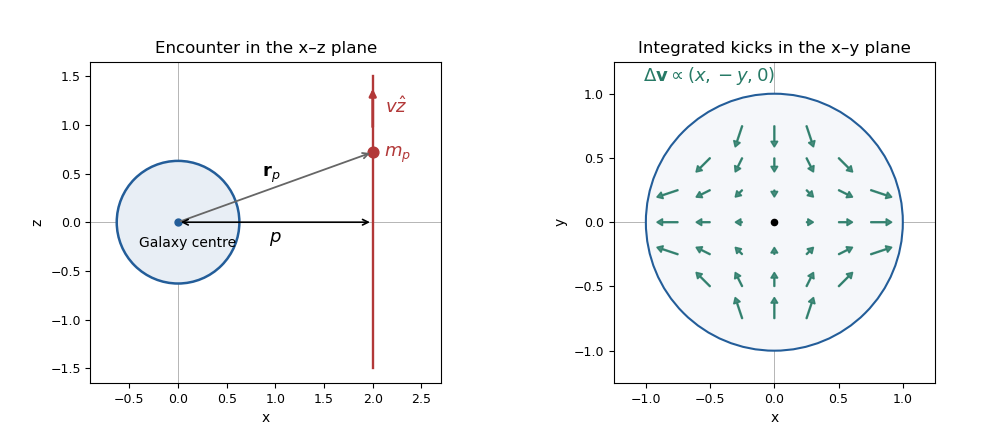
Write $\mathbf{u}$ for the star's initial velocity, distinguishing it from the perturber speed $v$. Its specific energy change is $\mathbf{u}\cdot \Delta \mathbf{v}+\frac{1}{2}|\Delta \mathbf{v}{|}^2$. The no-correlation assumption removes the first term on averaging; it is not an identity for every individual star. The mean specific heating at a given position is thereforeFor a spherical target, the mass-weighted averages satisfy $⟨x^2⟩=⟨y^2⟩=⟨z^2⟩=⟨r^2⟩/3$. The tidal impulse heating of a spherical galaxy is consequentlyHere $⟨r^2⟩=m_g^{-1}\int r^2\rho d^{3}r$ is assumed finite. Notice the change from specific energy to total energy after multiplying by $m_g$.

For two equal targets, each gains the same internal energy, so $\Delta U_{\mathrm{tot}}=8G^2{m}_g^3⟨r^2⟩/(3v^2{p}^4)$. Their relative-motion reduced mass is $m_g/2$. If $v$ denotes their relative speed at infinity, their initial orbital energy is $E_{\mathrm{orb}}=\frac{1}{2}(m_g/2)v^2=m_g{v}^2/4$. Internal tidal heating comes from this orbital energy. In the tidal capture of galaxies model, capture occurs if $\Delta U_{\mathrm{tot}}>E_{\mathrm{orb}}$, which gives the equal-mass tidal-capture thresholdCapture allows further passages and eventual merger in this simplified picture.

The encounter lasts roughly $p/v$. The impulse approximation needs $\Omega p/v\ll 1$, so that a star barely moves during the tide. When $v/p<\Omega$, stellar orbits respond during the perturbation and the kicks can cancel. Adiabatic invariance of an orbital action produces adiabatic shielding of tidal encounters, rather than the impulsive heating used above. The capture inequality cannot be extrapolated into that slow-encounter regime.

A rate-$\lambda$ Poisson process has $N_0=0$, right-continuous paths with upward jumps of size one, stationary independent increments, and $N_t-N_s\sim \mathrm{Poisson}(\lambda (t-s))$ for $t\ge s$. Assume $\lambda >0$. Its successive waiting times are independent exponential variables of rate $\lambda$. For $0<t_1<\cdots <t_n<t$, the product of their densities and the probability of no further jump before $t$ isDivide by $\mathbb{P}(N_t=n)=e^{-\lambda t}(\lambda t{)}^n/n!$ to obtain the conditional joint densityBoundary inequalities do not affect a density. Equivalently these are the ordered values of $n$ independent uniform points of $[0,t]$. For $n=0$, the conditional tuple is empty.

Consider a triangle of three links, each with capacity $C$. Calls for each pair of its three nodes arrive as independent Poisson processes at rate $\lambda$ and have independent holding times with an exponential distribution of mean one. Try the direct link first; if it is full, try the two-link path through the third node; if either alternative link is full, reject the call. This is alternative routing in a loss network.

In the symmetric Erlang fixed point approximation, let $B$ be each link's blocking probability. A given link receives direct offered traffic $\lambda$. Each of the other two call types contributes overflow traffic $\lambda B$, screened by the availability $1-B$ of the other link on its alternative path. ThusThe extra term expresses a feedback: blocking sends calls onto longer paths, which consume more total capacity and can create still more blocking.

Here is an explicit finite-capacity example, not just a limiting argument. Take $C=1000$ and $\lambda =950$, and let $F(B)=E(950[1+2B(1-B)],1000)-B$. Evaluating the Erlang loss formula givesThe displayed decimals are rounded, but the four signs can be checked exactly using the rational recursion $E(a,0)=1$, $E(a,k)=aE(a,k-1)/(k+aE(a,k-1))$. By the intermediate value theorem, there is a fixed point in each of $(0,0.01)$, $(0.01,0.1)$, and $(0.1,0.4)$. Numerically these three areThus alternative routing can produce multiple Erlang fixed points. This does not imply multiple stationary distributions for the exact finite continuous-time Markov chain, which is irreducible and has a unique stationary distribution; the multiplicity belongs to the approximation. The symmetric alternative-routing model is also discussed in Kelly's review of fixed point models of loss networks.